
In many cases an independent variable affects the outcome not only directly but also indirectly through another variable. We call the in-between variable a mediator.
Suppose that we want to know the relationship between Grade and Happiness. We may think that high grades directly increase happiness. Or there may be some other variable at play, such as Self-Esteem: high grades may not directly improve happiness, but may affect it through one’s self-esteem instead. For example, high grades increase self-esteem, and high self-esteem then increases happiness. In the latter case, self-esteem is the mediator that connects grades and happiness.
In a previous StatLab article, the author introduced a single mediator analysis and clearly demonstrated how to measure the indirect effect. Building on the single mediator analysis, this article extends it to two mediators, with a focus on parallel mediation.
We walk through the analysis using two approaches in R — simple linear regression with lm() and structural equation modeling with lavaan— and compare the process and their results. This article may be particularly useful if you are familiar with lm() but have not yet used lavaan. Lavaan makes mediation analysis considerably easier when multiple mediators are involved because it allows us to estimate all paths simultaneously and obtain standard errors and p-values for the indirect effects directly from the model syntax.
Parallel Mediation
When two mediators are involved, selecting an appropriate mediation model first requires determining the relationship between the mediators based on prior literature or theory—that is, whether they are independent or whether one influences the other. When one mediator influences the other, creating a sequential indirect pathway from the predictor to the outcome, such as X -> M1 -> M2 -> Y the model is called a serial mediation model. In contrast, when the two mediators independently transmit the predictor’s effect on the outcome, such as X -> M1 ->Y and X -> M2 -> Y, the model is called a parallel mediation model(Gervais et al., 2025). This article focuses on the parallel mediation model.
Let’s return to our imaginary example with two mediators. Suppose that Grade indirectly affects Happiness through two independent mediators, Social Recognition and Sense of Achievement. In this parallel mediation model, each mediator independently links the predictor to the outcome, but the two mediators are not strongly associated with each other. That is, Social Recognition is associated with Grade and Happiness, but not associated with Sense of Achievement, and vice versa, as illustrated in the following diagram.
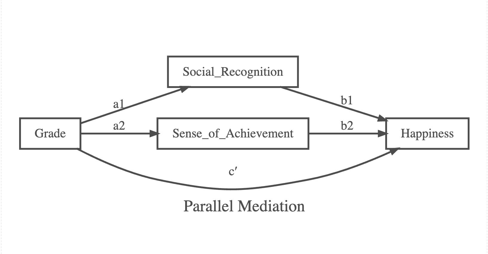
In the diagram, there are three pathways from Grade to Happiness: one direct pathway (\(c'\)) and two indirect pathways: One indirect pathway is through Social Recognition, and the other is through Sense of Achievement. Our main interest is to estimate the two specific indirect effects and the total indirect effect as their sum.
Each specific indirect effect is obtained by multiplying the two path coefficients along that pathway (Hayes, 2022).
- Specific indirect effect via M1: \(a_1 \times b_1\)
- Specific indirect effect via M2: \(a_2 \times b_2\)
- Total indirect effect: \((a_1 \times b_1) + (a_2 \times b_2)\)
- Total effect: \(c = c' + (a_1 \times b_1) + (a_2 \times b_2)\)
As a concrete example, let’s create a simulated dataset. The predictor X is drawn from a standard normal distribution. The two mediators are generated as linear functions of X with added noise: M1 is positively influenced by X (true \(a_1\) = 0.5) and M2 is negatively influenced by X (true \(a_2\) = −0.35). The outcome Y is generated as a linear combination of M1, M2, and X, with true coefficients \(b_1\) = −0.48, \(b_2\) = 0.7, and a small direct effect \(c'\) = 0.05. Since the true population effects are known, we can verify whether our model estimates close to these values.
# Set a random seed for reproducibility
set.seed(1984)

# Independent variable
X <- rnorm(100)

# Mediator 1: positively influenced by X
# True a1 = 0.5
M1 <- 0.5 * X + rnorm(100)

# Mediator 2: negatively influenced by X
# True a2 = -0.35
M2 <- -0.35 * X + rnorm(100)

# Outcome: influenced by both mediators
# True b1 (M1->Y) = -0.48, true b2 (M2->Y) = 0.7, and a small direct effect (X->Y)=0.05
Y <- -0.48 * M1 + 0.7 * M2 + 0.05*X + rnorm(100)

# Combine into a data frame
Data <- data.frame(X = X, Y = Y, M1 = M1, M2 = M2)

head(Data)
           X          Y         M1          M2
1  0.4092032 -0.3830332  0.4166264 -0.39137393
2 -0.3230250  0.2726644 -1.2934524  0.24741055
3  0.6358523 -0.9214520  0.7926085 -0.90959123
4 -1.8461288  1.2478553 -1.6501118 -0.04660574
5  0.9536474 -1.5640661  2.7996056 -0.61867564
6  1.1884898 -2.1487959 -0.0350344 -0.13551403
We know the true specific indirect effects through M1 and M2, where each indirect effect is the product of its two path coefficients. We expect the model to recover estimates close to these true values.
- Specific indirect effect via M1: 0.5 × (−0.48) = −0.24
- Specific indirect effect via M2: (−0.35) × 0.7 = −0.245
- Total indirect effect: (−0.24) + (−0.245) = −0.485
- Total effect: 0.05 + (−0.485) = −0.48
Now let’s implement mediation analysis both ways using a simple linear regression and SEM.
1. A simple linear regression approach using lm()
To estimate the indirect effects in a model with two parallel mediators, we fit three regression models1 to estimate the path coefficients \(a_1\), \(a_2\), \(b_1\), \(b_2\), and \(c'\) shown in the diagram above (Hayes, 2022). This framework is also used in the structural equation modeling approach introduced later.
\[M_1 = a_1 X\]
\[M_2 = a_2 X\]
\[Y = b_1 M_1 + b_2 M_2 + c' X\]
We now estimate each equation in turn.
First, M1 is regressed on X to estimate path \(a_1\).
# X predicts M1
model_m1 <- lm(M1 ~ X, data = Data)
summary(model_m1)
Call:
lm(formula = M1 ~ X, data = Data)

Residuals:
    Min      1Q  Median      3Q     Max
-2.5047 -0.6240 -0.0163  0.7126  2.3111

Coefficients:
            Estimate Std. Error t value Pr(>|t|)
(Intercept) -0.07594    0.09502  -0.799    0.426
X            0.59184    0.10139   5.838 6.88e-08 ***
---
Signif. codes:  0 '***' 0.001 '**' 0.01 '*' 0.05 '.' 0.1 ' ' 1

Residual standard error: 0.9497 on 98 degrees of freedom
Multiple R-squared:  0.258, Adjusted R-squared:  0.2504
F-statistic: 34.08 on 1 and 98 DF,  p-value: 6.875e-08
The result shows that X significantly predicts M1 with coefficient \(a_1\) = 0.59, which is close to the true value of 0.5.
Next, M2 is regressed on X to estimate path \(a_2\).
# X predicts M2
model_m2 <- lm(M2 ~ X, data = Data)
summary(model_m2)
Call:
lm(formula = M2 ~ X, data = Data)

Residuals:
    Min      1Q  Median      3Q     Max
-2.3991 -0.6389 -0.1305  0.6390  2.8594

Coefficients:
            Estimate Std. Error t value Pr(>|t|)
(Intercept) -0.14773    0.09579  -1.542    0.126
X           -0.12508    0.10220  -1.224    0.224

Residual standard error: 0.9573 on 98 degrees of freedom
Multiple R-squared:  0.01505,   Adjusted R-squared:  0.005004
F-statistic: 1.498 on 1 and 98 DF,  p-value: 0.2239
Unexpectedly, the effect of X on M2 is not statistically significant (\(a_2\) = −0.12, p = .22). This is likely because the sample size of 100 is not large enough to reliably detect the true effect of −0.35.
Lastly, Y is regressed on M1, M2, and X simultaneously to estimate path \(b_1\), \(b_2\) and \(c'\).
#  Both mediators and X predict Y
model_y<- lm(Y ~ M1 + M2 + X, data = Data)
summary(model_y)
Call:
lm(formula = Y ~ M1 + M2 + X, data = Data)

Residuals:
     Min       1Q   Median       3Q      Max
-2.31033 -0.61175 -0.07396  0.67214  2.21325

Coefficients:
            Estimate Std. Error t value Pr(>|t|)
(Intercept)   0.0121     0.1014   0.119    0.905
M1           -0.4586     0.1072  -4.277 4.47e-05 ***
M2            0.6158     0.1064   5.789 8.89e-08 ***
X            -0.0699     0.1257  -0.556    0.580
---
Signif. codes:  0 '***' 0.001 '**' 0.01 '*' 0.05 '.' 0.1 ' ' 1

Residual standard error: 0.9995 on 96 degrees of freedom
Multiple R-squared:  0.3906,    Adjusted R-squared:  0.3715
F-statistic: 20.51 on 3 and 96 DF,  p-value: 2.376e-10
- M1 predicts Y with coefficient \(b_1\) = −0.46,
- M2 predicts Y with coefficient \(b_2\) = 0.62,
- The direct effect of X on Y is not statistically significant (\(c'\) = −0.07, p = .58).
Now we have all the path coefficients for calculating the indirect, direct, and total effects.
The specific indirect effects are:
- via M1: \(a_1\) × \(b_1\) = 0.59 × (−0.46) = −0.27
- via M2: \(a_2\) × \(b_2\) = (−0.13) × 0.62 = −0.08
Thus, the total indirect effect is the sum of the two specific indirect effects: (−0.27) + (−0.08) = −0.35. The total effect of X on Y is then the sum of the direct effect and total indirect effect:(−0.07) + (−0.35) = −0.42. This total effect of X is equivalent to the coefficient estimated by regressing Y on X alone, which we can verify directly as shown below.
summary(lm(Y~X, data = Data))
Call:
lm(formula = Y ~ X, data = Data)

Residuals:
    Min      1Q  Median      3Q     Max
-2.6627 -0.8328  0.2156  0.8264  2.6235

Coefficients:
            Estimate Std. Error t value Pr(>|t|)
(Intercept) -0.04404    0.12044  -0.366  0.71544
X           -0.41836    0.12851  -3.255  0.00156 **
---
Signif. codes:  0 '***' 0.001 '**' 0.01 '*' 0.05 '.' 0.1 ' ' 1

Residual standard error: 1.204 on 98 degrees of freedom
Multiple R-squared:  0.09759,   Adjusted R-squared:  0.08838
F-statistic:  10.6 on 1 and 98 DF,  p-value: 0.001555
It is worth noting that the significant total effect of X (c = −0.42) becomes non-significant when both mediators are included in the model (c’ = −0.07, p > .05). This is consistent with the mediation criteria outlined by Baron & Kenny (1986): the direct effect of X weakens substantially once the mediators are included.
Confidence intervals for indirect effects
While the point estimates give us the magnitude of the indirect effects, they do not tell us whether these effects are statistically significant. To evaluate statistical significance, we need confidence intervals and p-values for the indirect effects. Hayes (2022) suggests that bootstrapping is preferable for constructing confidence intervals over the normal theory approach, as it does not assume a specific sampling distribution and tends to be more powerful than competing methods such as the Sobel test.
Although lm() provides estimates and confidence intervals for individual regression coefficients, it does not directly provide confidence intervals for manually defined indirect effects, such as products of coefficients. Therefore, we extract the relevant path coefficients from the three regression models and use nonparametric bootstrapping to construct confidence intervals for the specific indirect effects and the total indirect effect. If a bootstrap confidence interval does not include zero, the corresponding indirect effect is considered statistically significant.
Note that this article focuses on the overall process of parallel mediation analysis, so we present the bootstrapping code with brief descriptions only. For a detailed step-by-step explanation of how bootstrapping works and how to implement it using the boot package, see this supplementary document.
library(boot)

#1. Define the bootstrap function
boot_fn <- function(data, indices) {
  d <- data[indices, ]

  # Fit the 3 regression models for the mediation paths
  m1 <- lm(M1 ~ X, data = d)
  m2 <- lm(M2 ~ X, data = d)
  y  <- lm(Y ~ M1 + M2 + X, data = d)
  # Fit the total effect model
  total_model <- lm(Y ~ X, data = d)

  # Extract path coefficient estimates
  a1 <- coef(m1)["X"]
  a2 <- coef(m2)["X"]
  b1 <- coef(y)["M1"]
  b2 <- coef(y)["M2"]
  cp <- coef(y)["X"]
  c_total <- coef(total_model)["X"]

  # Define the indirect effects
  ind_m1  <- a1 * b1
  ind_m2  <- a2 * b2
  tot_ind <- ind_m1 + ind_m2

  # Return the effects to be bootstrapped
  c(
    ind_m1 = ind_m1,
    ind_m2 = ind_m2,
    total_indirect = tot_ind,
    direct_effect = cp,
    total_effect = c_total
  )
}

#2. Run the bootstrap
set.seed(123)

boot_res <- boot(
  data = Data,
  statistic = boot_fn,
  R = 5000
)

#3. Extract percentile bootstrap confidence intervals
get_ci <- function(i) {
  ci <- boot.ci(boot_res, type = "perc", index = i)
  round(ci$percent[4:5], 4)
}

# Apply the get_ci function to the 5 effects
ci_mat <- t(sapply(1:5, get_ci))

#4. Create a summary table
results_table <- data.frame(
  Path = c(
    "Indirect via M1 (a1*b1)",
    "Indirect via M2 (a2*b2)",
    "Total indirect effect",
    "Direct effect (c')",
    "Total effect (c)"
  ),

  Estimate = round(boot_res$t0, 4), #boot_res$t0 contains the original-sample estimates
  CI_lower = ci_mat[, 1],
  CI_upper = ci_mat[, 2]
)

#5. Determine significance based on whether the CI includes 0
results_table$Significant <- ifelse(
  results_table$CI_lower > 0 | results_table$CI_upper < 0,
  "Yes",
  "No"
)

rownames(results_table) <- NULL # Remove row names for a cleaner table
results_table
                     Path Estimate CI_lower CI_upper Significant
1 Indirect via M1 (a1*b1)  -0.2714  -0.4394  -0.1327         Yes
2 Indirect via M2 (a2*b2)  -0.0770  -0.2066   0.0327          No
3   Total indirect effect  -0.3485  -0.5701  -0.1695         Yes
4      Direct effect (c')  -0.0699  -0.3649   0.2236          No
5        Total effect (c)  -0.4184  -0.6929  -0.1682         Yes
The results show that the indirect effect via M1, the total indirect effect, and the total effect are statistically significant. However, the indirect effect via M2 is not statistically significant, as the path from X to M2 (\(a_2\)) is not significant. Now let’s examine whether the SEM approach produces the same results.
2. A structural equation modeling approach using sem()
Before we begin, it may be helpful to briefly review the three operators used to specify the mediation model in sem() from the lavaan package. For a complete list of operators, refer to Rosseel (2012).
~specifies a regression relationship. For example,Y ~ Xmeans thatYis regressed onX.~~specifies a covariance or variance. For example,M1 ~~ M2estimates the covariance betweenM1andM2.:=defines a new derived parameter. For example,indirect := a * bdefines the indirect effect as the product of pathsaandb.
As you can see, the same models and defined parameters used in the lm() approach are also used in the SEM approach. The key difference is that all equations are specified in a single syntax, and p-values and confidence intervals for the defined parameters are available by simply adding se = "bootstrap" to the sem() and ci = TRUE to summary().
Note that the coefficient labels in the sem() model (e.g., a, b, c) are arbitrary and can be named however you prefer. They are simply used to reference paths when calculating indirect and total effects.
library(lavaan)
# specify the parallel mediation model syntax

model_parallel <- '
  M1 ~ a1 * X
  M2 ~ a2 * X
  Y  ~ b1 * M1 + b2 * M2 + c * X

  indirect1      := a1 * b1
  indirect2      := a2 * b2
  total_indirect := indirect1 + indirect2
  total          := c + total_indirect
'

# estimate the model using maximum likelihood

fit_parallel <- sem(model_parallel,
                    data = Data,
                    se = "bootstrap") # use bootstrapping for SE

summary(fit_parallel,
        ci = TRUE) # include confidence intervals
lavaan 0.6-20 ended normally after 1 iteration

  Estimator                                         ML
  Optimization method                           NLMINB
  Number of model parameters                         8

  Number of observations                           100

Model Test User Model:

  Test statistic                                 1.706
  Degrees of freedom                                 1
  P-value (Chi-square)                           0.191

Parameter Estimates:

  Standard errors                            Bootstrap
  Number of requested bootstrap draws             1000
  Number of successful bootstrap draws            1000

Regressions:
                   Estimate  Std.Err  z-value  P(>|z|) ci.lower ci.upper
  M1 ~
    X         (a1)    0.592    0.091    6.530    0.000    0.423    0.780
  M2 ~
    X         (a2)   -0.125    0.090   -1.388    0.165   -0.294    0.054
  Y ~
    M1        (b1)   -0.459    0.102   -4.512    0.000   -0.672   -0.253
    M2        (b2)    0.616    0.105    5.886    0.000    0.399    0.816
    X          (c)   -0.070    0.148   -0.474    0.636   -0.371    0.211

Variances:
                   Estimate  Std.Err  z-value  P(>|z|) ci.lower ci.upper
   .M1                0.884    0.128    6.931    0.000    0.626    1.133
   .M2                0.898    0.134    6.688    0.000    0.638    1.167
   .Y                 0.959    0.123    7.770    0.000    0.684    1.182

Defined Parameters:
                   Estimate  Std.Err  z-value  P(>|z|) ci.lower ci.upper
    indirect1        -0.271    0.077   -3.521    0.000   -0.435   -0.136
    indirect2        -0.077    0.059   -1.312    0.189   -0.198    0.030
    total_indirect   -0.348    0.101   -3.459    0.001   -0.567   -0.166
    total            -0.418    0.131   -3.182    0.001   -0.687   -0.174
As expected, all estimates are very close to those obtained from the lm() approach. However, even though the significance conclusions remain unchanged, the p-values slightly differ because the two approaches use different methods for calculating standard errors2 and test statistics: sem() uses z-tests whereas lm() uses t-tests.
The variances in SEM output correspond to the squared residual standard errors in the lm() approach. They are slightly smaller than those from lm(). The gap decreases as sample size increases.
If you want a more concise summary of the results, the parameterEstimates() function is useful.
parameterEstimates(fit_parallel)
              lhs op                 rhs          label    est    se      z
1              M1  ~                   X             a1  0.592 0.091  6.530
2              M2  ~                   X             a2 -0.125 0.090 -1.388
3               Y  ~                  M1             b1 -0.459 0.102 -4.512
4               Y  ~                  M2             b2  0.616 0.105  5.886
5               Y  ~                   X              c -0.070 0.148 -0.474
6              M1 ~~                  M1                 0.884 0.128  6.931
7              M2 ~~                  M2                 0.898 0.134  6.688
8               Y ~~                   Y                 0.959 0.123  7.770
9               X ~~                   X                 0.877 0.000     NA
10      indirect1 :=               a1*b1      indirect1 -0.271 0.077 -3.521
11      indirect2 :=               a2*b2      indirect2 -0.077 0.059 -1.312
12 total_indirect := indirect1+indirect2 total_indirect -0.348 0.101 -3.459
13          total :=    c+total_indirect          total -0.418 0.131 -3.182
   pvalue ci.lower ci.upper
1   0.000    0.423    0.780
2   0.165   -0.294    0.054
3   0.000   -0.672   -0.253
4   0.000    0.399    0.816
5   0.636   -0.371    0.211
6   0.000    0.626    1.133
7   0.000    0.638    1.167
8   0.000    0.684    1.182
9      NA    0.877    0.877
10  0.000   -0.435   -0.136
11  0.189   -0.198    0.030
12  0.001   -0.567   -0.166
13  0.001   -0.687   -0.174
Another thing SEM can do is explicitly account for covariances between variables of interest. For example, we may check whether M1 and M2 somewhat are related — think of the relationship between Social Recognition and Sense of Achievement, which could move together. In this case, we can add their covariance to the model using M1 ~~ M2, although we do not expect them to be related in our simulated data.
Here, we create another model by simply adding the covariance term to model_parallel with the paste() function and refitting the model.
model_parallel_cov <- paste( model_parallel,
                            "M1 ~~ M2" )

fit_parallel_cov <- sem(model_parallel_cov,
                        data = Data,
                        se = "bootstrap")


summary(fit_parallel_cov ,
        ci = TRUE) # include confidence intervals
lavaan 0.6-20 ended normally after 9 iterations

  Estimator                                         ML
  Optimization method                           NLMINB
  Number of model parameters                         9

  Number of observations                           100

Model Test User Model:

  Test statistic                                 0.000
  Degrees of freedom                                 0

Parameter Estimates:

  Standard errors                            Bootstrap
  Number of requested bootstrap draws             1000
  Number of successful bootstrap draws            1000

Regressions:
                   Estimate  Std.Err  z-value  P(>|z|) ci.lower ci.upper
  M1 ~
    X         (a1)    0.592    0.091    6.530    0.000    0.423    0.780
  M2 ~
    X         (a2)   -0.125    0.090   -1.388    0.165   -0.294    0.054
  Y ~
    M1        (b1)   -0.459    0.102   -4.512    0.000   -0.672   -0.253
    M2        (b2)    0.616    0.105    5.886    0.000    0.399    0.816
    X          (c)   -0.070    0.148   -0.474    0.636   -0.371    0.211

Covariances:
                   Estimate  Std.Err  z-value  P(>|z|) ci.lower ci.upper
 .M1 ~~
   .M2                0.116    0.100    1.154    0.248   -0.082    0.312

Variances:
                   Estimate  Std.Err  z-value  P(>|z|) ci.lower ci.upper
   .M1                0.884    0.128    6.931    0.000    0.626    1.133
   .M2                0.898    0.134    6.688    0.000    0.638    1.167
   .Y                 0.959    0.123    7.770    0.000    0.684    1.182

Defined Parameters:
                   Estimate  Std.Err  z-value  P(>|z|) ci.lower ci.upper
    indirect1        -0.271    0.077   -3.521    0.000   -0.435   -0.136
    indirect2        -0.077    0.059   -1.312    0.189   -0.198    0.030
    total_indirect   -0.348    0.101   -3.459    0.001   -0.567   -0.166
    total            -0.418    0.131   -3.182    0.001   -0.687   -0.174
As expected, the covariance between M1 and M2 is small and non-significant, leaving all other estimates unchanged.
Visualizing the Path Diagram
Lastly, you can visualize the path with lavaanPlot()
library(lavaanPlot)
lavaanPlot(model  = fit_parallel,  # the fitted lavaan model object
           coefs  = TRUE,           # display path coefficients on the arrows
           stand  = FALSE,          # use unstandardized coefficients
           sig    = 0.05,         # only show paths with p < .05
           graph_options = list(rankdir = "LR"),  # left to right layout
           node_options  = list(fontsize = "12"), # node text size
           edge_options  = list(fontsize = "10")) # path coefficient text size
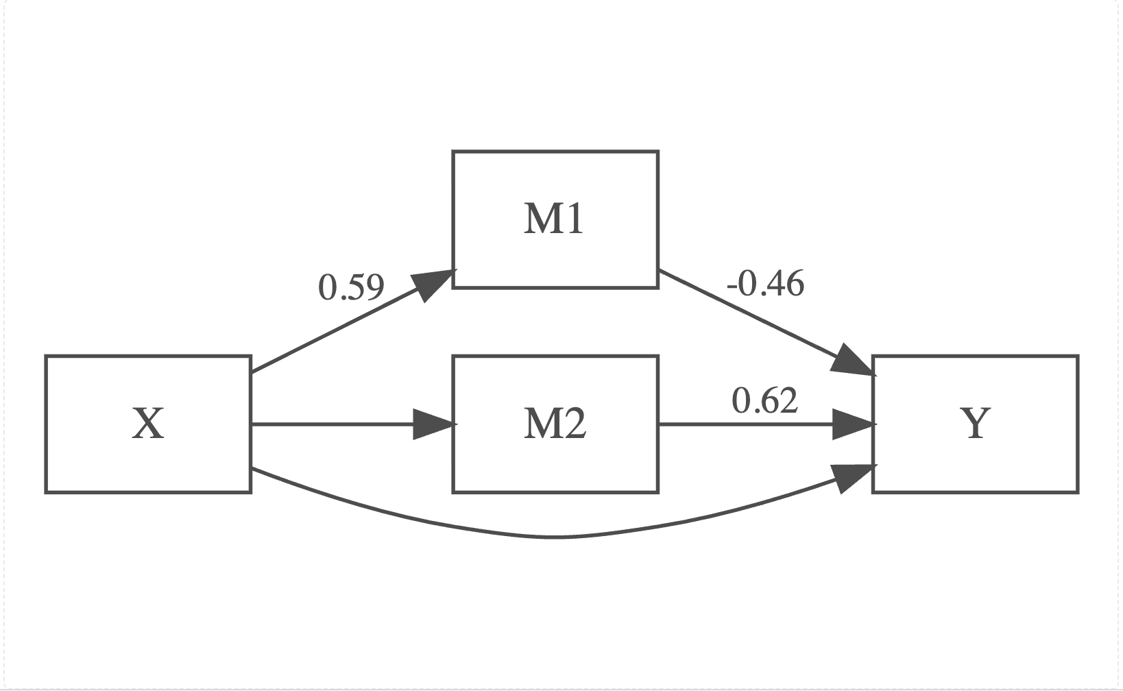
The path diagram displays only the statistically significant paths (p < .05). X predicts M1 (\(a_1\) = 0.59), which in turn negatively predicts Y (\(b_1\) = −0.46), indicating a significant indirect effect of X on Y through M1. M2 positively predicts Y (\(b_2\) = 0.62); however, the path from X to M2 is not significant, resulting in a non significant indirect effect through M2. The direct path from X to Y is also absent. This indicates that the effect of X on Y operates primarily through M1.
Note that we know the true effect of X on M2 exists (\(a_2\) = −0.35) based on our simulation, but it was not detected here likely due to insufficient statistical power with a sample size of n = 100. With a larger sample size, the estimates would become more accurate and the true effect would likely be detected.
R session details
All analyses were performed in R (v4.5.1; R Core Team, 2025) on macOS Sequoia (Apple M1 Pro), using the packages boot (v1.3.31), lavaan (v0.6-20; Rosseel, 2012), and lavaanPlot (v0.8.1).
Acknowledgement
Generative AI (Claude Sonnet) assisted with editing for clarity and grammar. AI generated codes for bootstrapping is subsequently reviewed, tested, and refined by the author. I also thank Clay for providing a detailed supplemental explanation of the bootstrapping process.
References
- Baron, R. M., & Kenny, D. A. (1986). The moderator–mediator variable distinction in social psychological research: Conceptual, strategic, and statistical considerations. Journal of Personality and Social Psychology, 51(6), 1173–1182.https://doi.org/10.1037/0022-3514.51.6.1173
- Canty A, Ripley B (2025). boot: Bootstrap Functions. doi:10.32614/CRAN.package.boot https://doi.org/10.32614/CRAN.package.boot. R package version 1.3-32 https://CRAN.R-project.org/package=boot.
- Gervais, J., Lefebvre, G., & Moodie, E. E. M. (2025). Causal mediation analysis with two mediators: A comprehensive guide to estimating total and natural effects across various multiple mediators setups. Psychological Methods. Advance online publication. https://doi.org/10.1037/met0000781
- Hayes, A. F. (2022). Introduction to mediation, moderation, and conditional process analysis: A regression-based approach (3rd ed.). The Guilford Press.
- Kim, B. (2016). Introduction to mediation analysis. University of Virginia Library StatLab. https://library.virginia.edu/data/articles/introduction-to-mediation-analysis
- Lishinski A (2024). lavaanPlot: Path Diagrams for ‘Lavaan’ Models via ‘DiagrammeR’. doi:10.32614/CRAN.package.lavaanPlot https://doi.org/10.32614/CRAN.package.lavaanPlot. R package version 0.8.1, https://CRAN.R-project.org/package=lavaanPlot.
- R Core Team. (2025). R: A language and environment for statistical computing. R Foundation for Statistical Computing. https://www.R-project.org/
- Rosseel, Y. (2012). lavaan: An R package for structural equation modeling. Journal of Statistical Software, 48(2), 1–36. https://www.jstatsoft.org/article/view/v048i02
Hyeseon Seo
Statistical Research Consultant
University of Virginia Library
May 20, 2026
- Intercepts and error terms are omitted from the equations for clarity, following standard path diagram notation.↩︎
lm()uses Ordinary Least Squares (OLS) and divides the residual sum of squares by n − k − 1, while SEM uses Maximum Likelihood (ML) and divides by n, where k = number of predictors and n = number of observations. This is whylm()gives slightly larger variance estimates.↩︎
For questions or clarifications regarding this article, contact statlab@virginia.edu.
View the entire collection of UVA Library StatLab articles, or learn how to cite.