Understanding ICC

Investigating ICC through simulation

A good way to get acquainted with the ICC is to simulate and visualize data. Below we generate five observations each for ten arbitrary groups and then look at the first six rows. Here each “group” could represent a single person we observed on five consecutive days, or a single tree on which we collected five observations.

d <- expand.grid(obs = 1:5,grp = factor(1:10))
head(d)

  obs grp
1   1   1
2   2   1
3   3   1
4   4   1
5   5   1
6   1   2

Now let’s simulate data for these ten groups with two sources of variation:

1. within-group
2. between-group

The within-group variation is created by drawing 50 values from a normal distribution with mean 0 and standard deviation 0.2. The between-group variation is created by drawing 10 values (one for each group) from a normal distribution with mean 0 and standard deviation 1.8. We then generate data for each group by starting with the value 2 and adding both between and within variation to it. The syntax between[d$grp] repeats each of the ten “between” values five times for each group. The set.seed() function makes our randomly generated values reproducible. If you run the following chunk of code with set.seed(1) then you will generate the same data.

set.seed(1)
within <- rnorm(n = nrow(d), mean = 0, sd = 0.2)
between <- rnorm(n = 10, mean = 0, sd = 1.8)
d$y <- (2 + between[d$grp]) + within

We can visualize the variation within and between groups with a strip chart. Below we use the ggplot2 package to create the plot. If you don’t have the ggplot2 package, or any other package used in this article, you can install them using the install.packages() function. For example, install.packages("ggplot2").

library(ggplot2)
ggplot(d) +
  aes(x = grp, y = y) +
  geom_point()

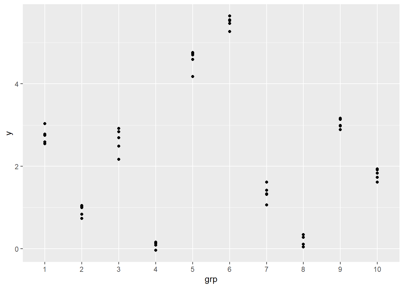
Notice the between-group variation is relatively large compared to the within-group variation. We can see that the between group variation ranges about six units on the y axis while the within group variation ranges about one unit on the y axis at most. Most of the variation in y is due to variation between groups. How much of the total variation in y is due to the variation between groups? This is what ICC summarizes.

Let’s fit a mixed-effect model to this data and calculate the ICC. To do this we’ll use the lmer() function from the lme4 package (Bates et al., 2015). The formula syntax below says to model y with just an intercept, but to make the intercept conditional on the group. This will estimate a model with an overall intercept, but with separate intercepts fit to each group.

library(lme4)
m <- lmer(y ~ 1 + (1|grp), data = d)
summary(m)

Linear mixed model fit by REML ['lmerMod']
Formula: y ~ 1 + (1 | grp)
   Data: d

REML criterion at convergence: 30.3

Scaled residuals: 
    Min      1Q  Median      3Q     Max 
-2.5150 -0.5807  0.1304  0.6049  1.6515 

Random effects:
 Groups   Name        Variance Std.Dev.
 grp      (Intercept) 3.210    1.7917  
 Residual             0.032    0.1789  
Number of obs: 50, groups:  grp, 10

Fixed effects:
            Estimate Std. Error t value
(Intercept)   2.2783     0.5672   4.017

In the output under “Fixed Effects” we see the overall intercept is estimated as 2.2783, which is close to the true value of 2 we used to simulate the data. More relevant to this article, under “Random Effects” we see the estimated between-group variance (3.210) and the estimated within-group variance (0.032). The ICC is calculated by dividing the between-group variance by the sum of the two variances. This produces a value that can range from 0 to 1. The ICC for our example comes out to about 0.99. About 99% of the variability in y is due to the variation between groups.

3.210/(3.210 + 0.032)

[1] 0.9901295

Since we simulated this data we can calculate the true ICC. Above we simulated within- and between-group variances by drawing from normal distributions with standard deviations of 0.2 and 1.8, respectively. The true ICC is then calculated by squaring the values to get variance.

1.8^2/(1.8^2 + 0.2^2)

[1] 0.9878049

We can also use the icc() function from the performance package to calculate ICC (Lüdecke et al., 2021).

library(performance)
icc(m)

# Intraclass Correlation Coefficient

    Adjusted ICC: 0.990
  Unadjusted ICC: 0.990

Notice it returns two estimates of ICC, adjusted and unadjusted. The documentation for the icc() function explains the difference: “While the adjusted ICC only relates to the random effects, the unadjusted ICC also takes the fixed effects variances into account, more precisely, the fixed effects variance is added to the denominator of the formula to calculate the ICC.”

Since our example has no fixed effects (i.e., no predictors) both the adjusted and unadjusted estimates are the same. (We explain more about unadjusted ICC below.)

We can get more insight into the ICC by looking at the group-specific intercepts, which we can view using the coef() function.

coef(m)

$grp
   (Intercept)
1   2.74152113
2   0.92807140
3   2.62095696
4   0.06347521
5   4.59107816
6   5.48860453
7   1.34936121
8   0.16455568
9   3.02987647
10  1.80561930

attr(,"class")
[1] "coef.mer"

Notice the wide variability in the estimated intercepts. Some are close to 0 and others are over 4. Each of these intercepts are essentially estimating the mean y value for each group.

Example of low ICC

Now let’s simulate data with a low ICC. We can use our code above and simply switch the values for sd in the rnorm() functions.

set.seed(4)
within <- rnorm(n = nrow(d), mean = 0, sd = 1.8)
between <- rnorm(n = 10, mean = 0, sd = 0.2)
d$y <- (2 + between[d$grp]) + within

The true ICC in this case is about 0.01.

0.2^2/(0.2^2 + 1.8^2)

[1] 0.01219512

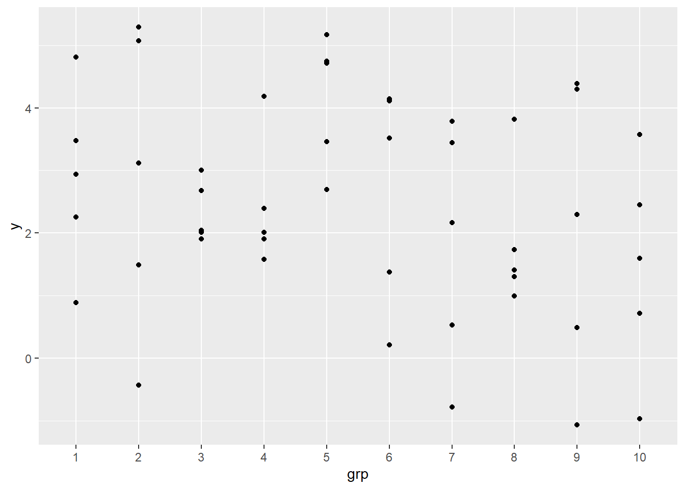
When we plot the data we see each group has about the same variation and the same range. Most of the variation in this data is due to variation within the groups.

ggplot(d) +
  aes(x = grp, y = y) +
  geom_point()

Fitting a mixed-effect model to this data shows a small estimated between-group variance (0.03326) and a large estimated within-group variance (2.72359).

m2 <- lmer(y ~ 1 + (1|grp), data = d)
summary(m2)

Linear mixed model fit by REML ['lmerMod']
Formula: y ~ 1 + (1 | grp)
   Data: d

REML criterion at convergence: 192.6

Scaled residuals: 
     Min       1Q   Median       3Q      Max 
-2.12449 -0.61037 -0.06216  0.79592  1.69960 

Random effects:
 Groups   Name        Variance Std.Dev.
 grp      (Intercept) 0.03326  0.1824  
 Residual             2.72359  1.6503  
Number of obs: 50, groups:  grp, 10

Fixed effects:
            Estimate Std. Error t value
(Intercept)   2.4583     0.2404   10.22

The ICC in this case is estimated to be about 0.01, similar to what we calculated above using the true variance values.

0.03326/(0.03326 + 2.72359)

[1] 0.01206449

Or using the icc() function:

icc(m2)

# Intraclass Correlation Coefficient

    Adjusted ICC: 0.012
  Unadjusted ICC: 0.012

Looking at the group-specific intercepts reveals little variability between the groups. All but one is estimated to be about 2.4.

coef(m2)

$grp
   (Intercept)
1     2.482185
2     2.484122
3     2.450744
4     2.455668
5     2.555956
6     2.470485
7     2.422011
8     2.423299
9     2.436491
10    2.401582

attr(,"class")
[1] "coef.mer"

Example of singular model fit

Sometimes fitting models to data that have little between-group variability can result in “singular” fits. This means the between-group variance is estimated as 0, which is the lower bound of possible values for variance. By changing the seed in our previous example, we can generate such a result.

set.seed(2)
within <- rnorm(n = nrow(d), mean = 0, sd = 1.8)
between <- rnorm(n = 10, mean = 0, sd = 0.2)
d$y <- (2 + between[d$grp]) + within
m3 <- lmer(y ~ 1 + (1|grp), data = d)

boundary (singular) fit: see help('isSingular')

Looking at the model summary shows the between group variance estimated as 0.

summary(m3)

Linear mixed model fit by REML ['lmerMod']
Formula: y ~ 1 + (1 | grp)
   Data: d

REML criterion at convergence: 212.9

Scaled residuals: 
     Min       1Q   Median       3Q      Max 
-2.43965 -0.66565 -0.01258  0.68941  1.86921 

Random effects:
 Groups   Name        Variance Std.Dev.
 grp      (Intercept) 0.000    0.00    
 Residual             4.163    2.04    
Number of obs: 50, groups:  grp, 10

Fixed effects:
            Estimate Std. Error t value
(Intercept)   2.1715     0.2885   7.526
optimizer (nloptwrap) convergence code: 0 (OK)
boundary (singular) fit: see help('isSingular')

Likewise, looking at the group-specific intercepts shows no variability whatsoever.

coef(m3)

$grp
   (Intercept)
1     2.171484
2     2.171484
3     2.171484
4     2.171484
5     2.171484
6     2.171484
7     2.171484
8     2.171484
9     2.171484
10    2.171484

attr(,"class")
[1] "coef.mer"

In cases like this we could say the estimated ICC is 0.

0/4.163

[1] 0

However, if we try using the icc() function on the fitted model object we get a missing value, NA, and a warning message.

icc(m3)

Warning: Can't compute random effect variances. Some variance components equal
  zero. Your model may suffer from singularity (see `?lme4::isSingular`
  and `?performance::check_singularity`).
  Decrease the `tolerance` level to force the calculation of random effect
  variances, or impose priors on your random effects parameters (using
  packages like `brms` or `glmmTMB`).

[1] NA

Since the estimated between-group variance is 0 (i.e., singular), the function refuses to calculate the ICC. However, it says we can try imposing “priors on your random effects parameters (using packages like brms or glmmTMB).” This basically means we can try to help the model estimate the between-group variance by encouraging it to look at a smaller range of values.

Here’s a quick example of how we could do this using the glmmTMB() function from the glmmTMB package (McGillycuddy et al, 2025). Notice the model syntax is the same. When we fit the model, we don’t get any “singular” warnings. However, the icc() function still doesn’t work.

library(glmmTMB)
m4 <- glmmTMB(y ~ 1 + (1|grp), data = d)
icc(m4)

Warning: Can't compute random effect variances. Some variance components equal
  zero. Your model may suffer from singularity (see `?lme4::isSingular`
  and `?performance::check_singularity`).
  Decrease the `tolerance` level to force the calculation of random effect
  variances, or impose priors on your random effects parameters (using
  packages like `brms` or `glmmTMB`).

[1] NA

To impose a prior distribution on the between-group variance, we specify a data frame with a prior distribution and a class label specifying which parameter the prior distribution is for. The glmmTMB package recommends using the gamma distribution for random effect prior distributions. The arguments to the gamma distribution are the mean and shape, respectively. We selected the distribution below, gamma(1, 2.5), based on examples in the glmmTMB priors vignette. With the prior data frame ready to go, we use the update() function to update the model and then call the icc() function.

prior <- data.frame(prior = "gamma(1, 2.5)",
                    class = "ranef")
m4 <- update(m4, priors = prior)
icc(m4)

# Intraclass Correlation Coefficient

    Adjusted ICC: 0.037
  Unadjusted ICC: 0.037

Another option is the rstanarm package which implements Bayesian modeling using familiar lme4 syntax (Goodrich et al, 2025). Below we use the stan_lmer() function to fit the mixed-effect model using rstanarm’s default prior distributions, and then call the icc() function on the fitted model object.

library(rstanarm)
m5 <- stan_lmer(y ~ 1 + (1|grp), data = d, refresh = 0)
icc(m5)

# Intraclass Correlation Coefficient

    Adjusted ICC: 0.065
  Unadjusted ICC: 0.065

Both estimates are slightly higher than the true ICC value of 0.01, but both are still small. Regardless of which approach we use, the same general conclusion is reached: there is little variation between groups. ¹

Unadjusted ICC

We mentioned earlier that the “unadjusted ICC also takes the fixed effects variances into account.” Let’s demonstrate what that means. Below we add a predictor to our data frame called “x”. Within each group, “x” ranges from 0 to 4. We then add “x” to the code that generates “y” and multiply it by 1.5.

d$x <- rep(0:4, 10)
set.seed(6)
within <- rnorm(n = nrow(d), mean = 0, sd = 0.4)
between <- rnorm(n = 10, mean = 0, sd = 1.4)
d$y <- (2 + between[d$grp]) + 1.5 * d$x + within

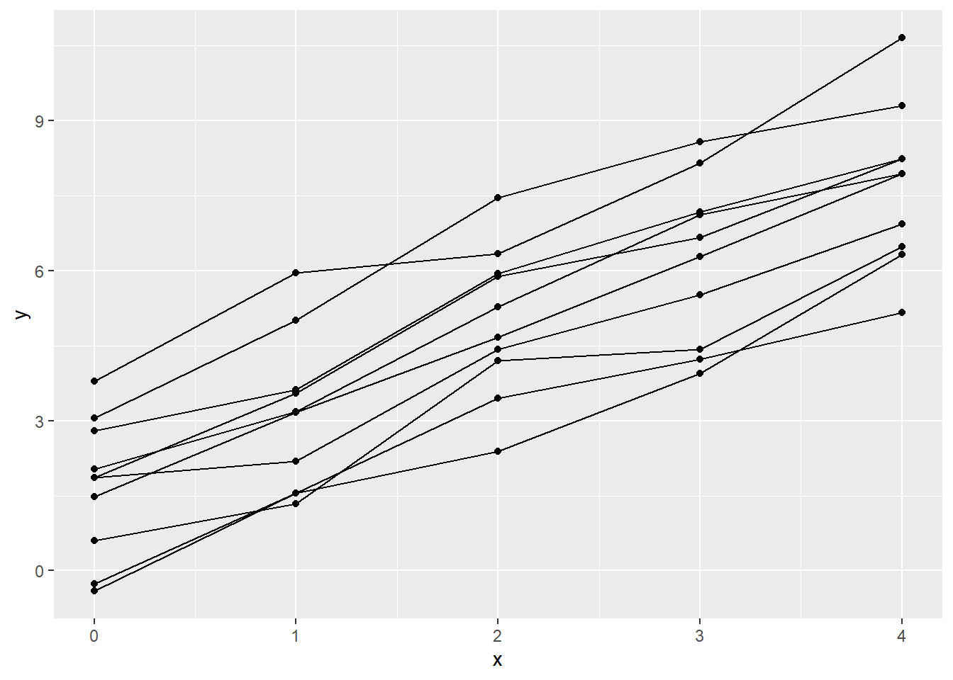
We visualize the data by plotting the points and connecting the points within each group. It should be obvious that some of the variability in “y” is now due to “x” as well as between and within groups.

ggplot(d) +
  aes(x, y, group = grp) +
  geom_point() +
  geom_line()

To model this data, we need to include “x” in our model formula. Since we simulated the data we know the correct model to fit: y ~ x + (1|grp). This says to model y as a function of x with an intercept that is conditional on group.

m6 <- lmer(y ~ x + (1|grp), data = d)
summary(m6, corr = FALSE)

Linear mixed model fit by REML ['lmerMod']
Formula: y ~ x + (1 | grp)
   Data: d

REML criterion at convergence: 104.1

Scaled residuals: 
    Min      1Q  Median      3Q     Max 
-1.6279 -0.7268 -0.1308  0.5909  1.8159 

Random effects:
 Groups   Name        Variance Std.Dev.
 grp      (Intercept) 2.1250   1.4577  
 Residual             0.2038   0.4514  
Number of obs: 50, groups:  grp, 10

Fixed effects:
            Estimate Std. Error t value
(Intercept)  1.70903    0.47405   3.605
x            1.51636    0.04514  33.591

Now the icc() function reports two different ICC values:

icc(m6)

# Intraclass Correlation Coefficient

    Adjusted ICC: 0.912
  Unadjusted ICC: 0.303

The adjusted ICC is what we described above: the between group variance divided by the sum of the variances.

2.1250/(2.1250 + 0.2038)

[1] 0.9124871

It’s called “adjusted” because it’s adjusted to only summarize the proportion of between-group variability within random effects.

The unadjusted ICC incorporates variability due to “x” in the denominator of the ICC calculation. This variability is estimated by multiplying each “x” value in the data frame by the model coefficient of “x” (1.51636) and then taking the variance of those values.

fixvar <- var(1.51636 * d$x)

Now add this value to the denominator to the ICC calculation to get the unadjusted ICC.

2.1250/(2.1250 + 0.2038 + fixvar)

[1] 0.3026485

This estimate of ICC is called “unadjusted” because it summarizes the proportion of between-group variability within both the random effects and the predictors. We expect it to be smaller since the denominator has an additional source of variability.

In most cases you’ll want to report the adjusted ICC. This is typically how ICC is defined in textbooks and and reported in journal articles. For example, see West et al (2015, page 118), Gelman and Hill (2007, page 258), and Singer and Willett (2003, page 96).

ICC in the presence of non-constant variance

One of the assumptions of mixed-effect/multilevel modeling is homoscedasticity, or constant variance of the residuals. This basically says the uncertainty in our model predictions is constant over the range of possible inputs. This can be assessed with residual versus fitted value plots. Calling plot() on a mixed-effect model object in R generates this plot. Below we demonstrate on our most recent model, m6.

plot(m6)

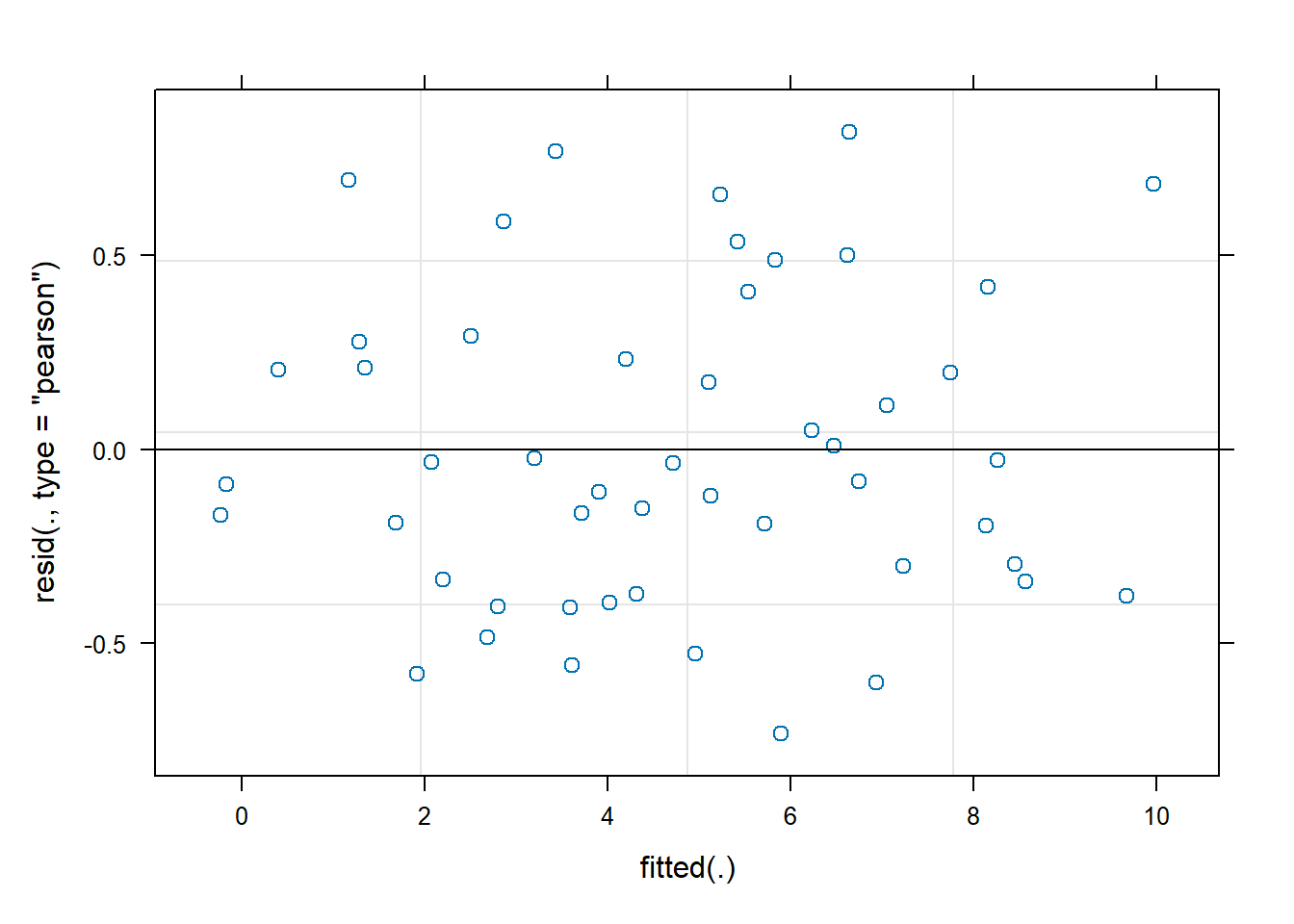
This plot looks good. The scatter around 0 on the y-axis as the fitted values increase along the x-axis stays constant. This tells us that the uncertainty in model-predicted values is constant no matter what we’re predicting.

Mixed-effect/multilevel models also assume constant variance within random effect groups. We can assess this assumption for model m6 using the following code.

plot(m6, grp ~ resid(.))

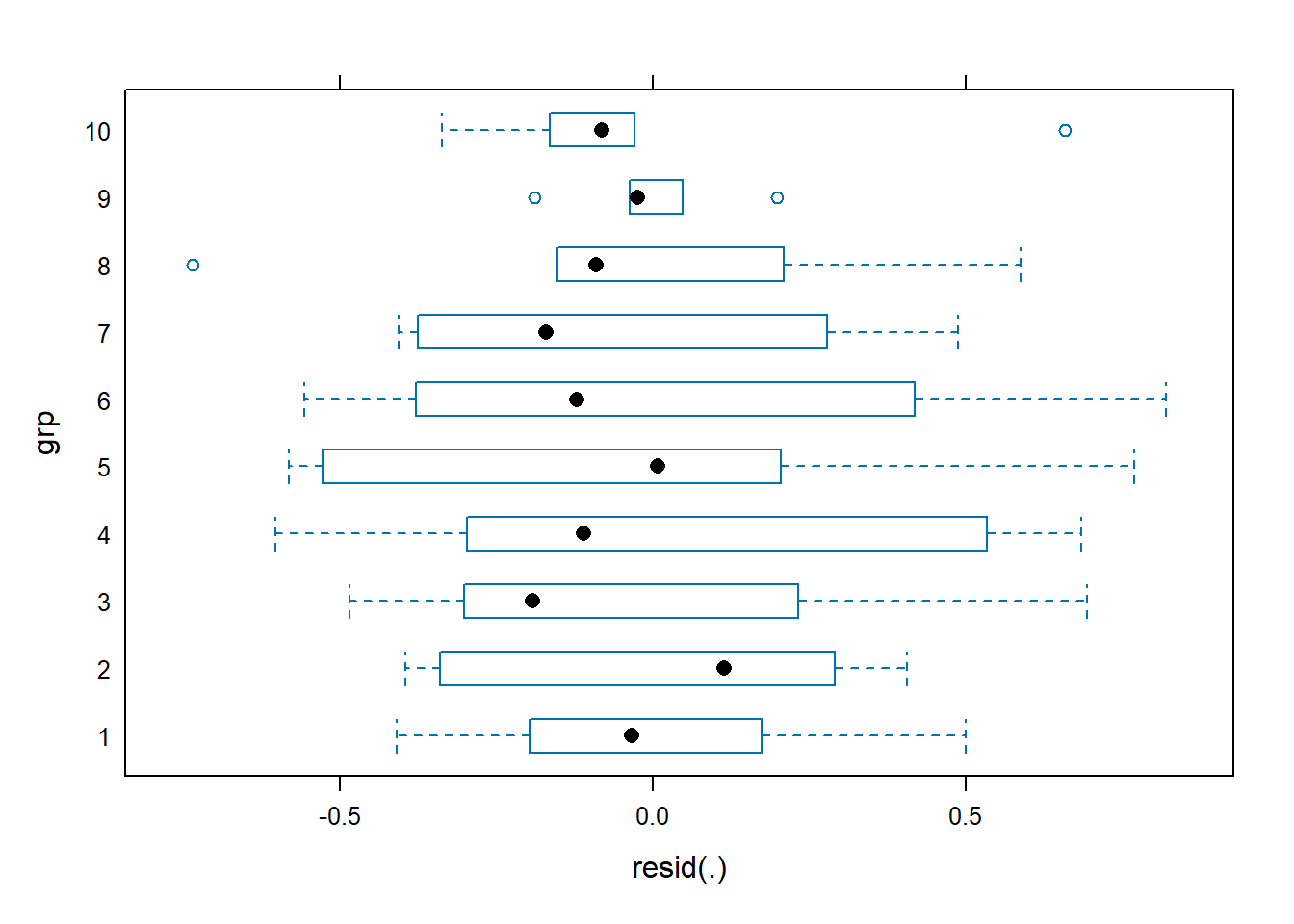
This plot looks pretty good as well. Within each group the residuals have a consistent scatter that mostly stays within 0.5 of 0.

But what if we have evidence of non-constant variance? How does this affect ICC? To investigate, let’s simulate data with non-constant variance. Below we generate a new variable called “trt” that takes the values 0 and 1. We then use that variable to create non-constant variance. Observations in groups 1 - 5 will have within variance simulated with a standard deviation of 0.4. Observations in groups 6 - 10 will have within variance simulated with a standard deviation of 2.4.

set.seed(10)
d$trt <- rep(0:1, each = 25)
within <- rnorm(n = nrow(d), mean = 0, 
                sd = ifelse(d$trt == 0, 0.4, 2.4))
between <- rnorm(n = 10, mean = 0, sd = 1.2)
d$y <- (2 + between[d$grp]) + 0.5 * (d$trt == 1) + within

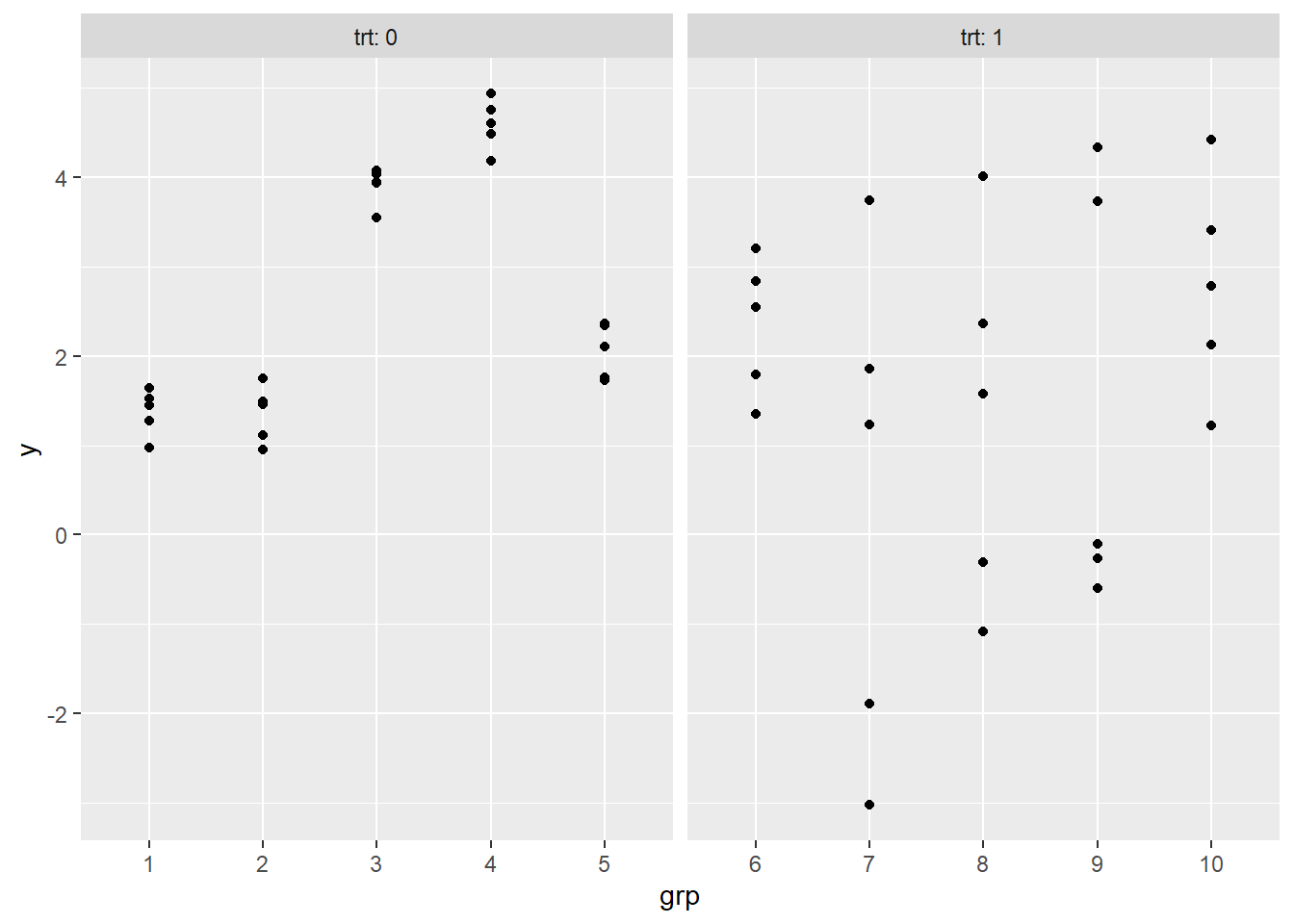
Plotting the data shows that observations with trt = 1 have a great deal more within-group variance than observations with trt = 0.

ggplot(d) +
  aes(grp, y) +
  geom_point() +
  facet_wrap(~trt, scales = "free_x", labeller = "label_both")

Modeling this data and looking at the scatter of residuals within groups reveals big problems.

m7 <- lmer(y ~ trt + (1|grp), data = d)
plot(m7, grp ~ resid(.))

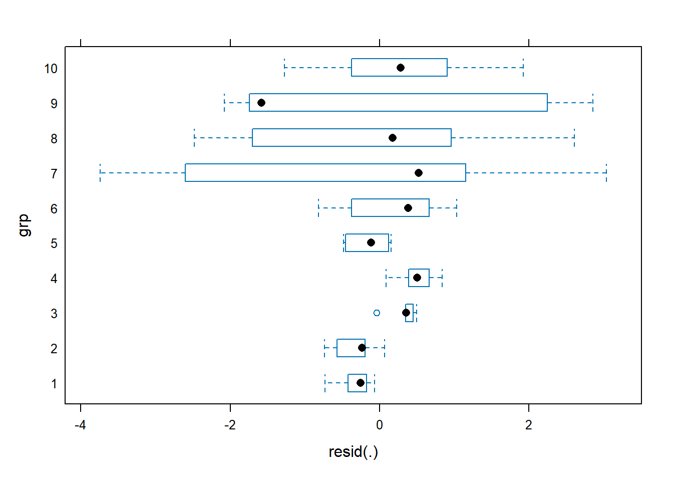
The adjusted ICC calculation for this model comes out to 0.367, but doesn’t seem meaningful based on our exploratory and diagnostic plots.

icc(m7)

# Intraclass Correlation Coefficient

    Adjusted ICC: 0.367
  Unadjusted ICC: 0.340

When trt = 0 it seems like ICC should be high. Likewise, when trt = 1 it seems like ICC should be low. It would be nice if we could calculate separate ICC values for the two levels of “trt”. Fortunately, we can do this by way of the lme() function in the nlme package that comes installed with R. The lme() function allows us to fit mixed-effect/multilevel models with separate within-group variances according to a specified grouping variable. Below the syntax weights = varIdent(form = ~ 1|trt) says to estimate separate within-group (i.e., residual) variances for the two groups of “trt”. Notice also that we have to specify the random effect grouping structure using random = ~ 1|grp. ²

library(nlme)
m8 <- lme(y ~ 1, data = d, random = ~ 1|grp, 
          weights = varIdent(form = ~ 1|trt))
summary(m8)

Linear mixed-effects model fit by REML
  Data: d 
       AIC      BIC    logLik
  147.3128 154.8801 -69.65641

Random effects:
 Formula: ~1 | grp
        (Intercept)  Residual
StdDev:    1.273959 0.2790434

Variance function:
 Structure: Different standard deviations per stratum
 Formula: ~1 | trt 
 Parameter estimates:
       0        1 
1.000000 6.996976 
Fixed effects:  y ~ 1 
               Value Std.Error DF t-value p-value
(Intercept) 2.247094 0.4407561 40 5.09827       0

Standardized Within-Group Residuals:
       Min         Q1        Med         Q3        Max 
-2.0534978 -0.9079523  0.1352652  0.5217969  1.4157339 

Number of Observations: 50
Number of Groups: 10 

In the summary output above we see a section titled “Variance function:” with a subheading that says “Structure: Different standard deviations per stratum”. This shows two estimates, one for trt = 0 and another for trt = 1. These are multipliers for the model residual standard deviation (0.2790434). The trt = 0 group is 1.0000, which implies the within-group variance for trt = 0 is simply \(0.2790434^2\). (We square the value since it’s expressed as a standard deviation.) The trt = 1 group is 6.996976. This implies the within-group variance for the trt = 1 group is \(0.2790434^2 \times 6.996976^2\). This multiplier is an estimate of the ratio of the trt = 1 standard deviation to the trt = 0 standard deviation. The true value is 6, which can be calculated from the standard deviations we used to simulate the within-group variance.

2.4/0.4

[1] 6

To calculate ICC for each group we use the same formula from above for the adjusted ICC. For the trt = 0 ICC, we divide the Intercept (between-group) variance by the sum of the Intercept and Residual (within-group) variances.

# trt = 0
1.273959^2 / (1.273959^2 + 0.2790434^2)

[1] 0.9542195

For the trt = 1 ICC, we do the same thing. But notice we need to multiply the Residual variance by the factor \(6.996976^2\).

# trt = 1
1.273959^2 / (1.273959^2 + (0.2790434^2 * 6.996976^2))

[1] 0.2986109

The ICCs are wildly different, but make sense according to the exploratory plot above. When trt = 0, most of the variance in y can be attributed to between-group differences. Hence the large ICC value of 0.95. When trt = 1, much of the variance in y can be attributed to within-group differences. Hence the smaller ICC value of 0.30.

While the icc() function cannot be used to calculate these separate ICCs, we can use the nlme function getVarCov() along with the cov2cor() function to view the marginal correlations of particular groups, which turns out to be the ICC. Below we get the marginal covariance matrix for group 1 (which is in the trt = 0 group) by setting individuals = "1" and specifying type = "marginal". We save the result and then use the cov2cor() function to convert the covariance matrix to a correlation matrix. The ICC is in the off diagonal. This matrix will have the same dimensions as the number of observations within a group. Since groups 2 - 5 also have five observations each and have trt = 0, their matrices will be identical to this one.

gvc <- getVarCov(m8, individuals = "1", type = "marginal")
cov2cor(gvc$`1`)

          1         2         3         4         5
1 1.0000000 0.9542194 0.9542194 0.9542194 0.9542194
2 0.9542194 1.0000000 0.9542194 0.9542194 0.9542194
3 0.9542194 0.9542194 1.0000000 0.9542194 0.9542194
4 0.9542194 0.9542194 0.9542194 1.0000000 0.9542194
5 0.9542194 0.9542194 0.9542194 0.9542194 1.0000000

If we look at the marginal correlations for group 6 (in the trt = 1 group), we get the other ICC.

gvc <- getVarCov(m8, individuals = "6", type = "marginal")
cov2cor(gvc$`6`)

          1         2         3         4         5
1 1.0000000 0.2986108 0.2986108 0.2986108 0.2986108
2 0.2986108 1.0000000 0.2986108 0.2986108 0.2986108
3 0.2986108 0.2986108 1.0000000 0.2986108 0.2986108
4 0.2986108 0.2986108 0.2986108 1.0000000 0.2986108
5 0.2986108 0.2986108 0.2986108 0.2986108 1.0000000

For this reason, the ICC is sometimes described as “a correlation coefficient between responses” in the same random effect group (West et al. 2015).

Final comments

ICC is usually not the primary focus of a mixed-effect/multilevel analysis. It’s a nice piece of additional information that summarizes how much variability in the outcome is due to random effect groups, but by itself it doesn’t tell us if we have a good model and should not be interpreted like an R-squared statistic.

One potential use of ICC is to determine if a mixed-effect/multilevel model is necessary. In this scenario, we fit an intercept-only model with random intercepts for the random effect groups, and then calculate the ICC. This type of model is sometimes called an unconditional means model because the predicted mean is not conditional on any predictors (Singer and Willett, 2003, Chapter 4). A very low value of ICC (close to 0) for this model indicates that the random effect groups are not explaining much of the variability in the outcome and that we might be able to get away with fitting a basic linear model. This is essentially what we did in the section “Example of low ICC”.

R session details

The analysis was done using the R Statistical language (v4.6.0; R Core Team, 2026) on Windows 11 x64, using the packages lme4 (v2.0.1), Matrix (v1.7.5), glmmTMB (v1.1.14), Rcpp (v1.1.1.1.1), rstanarm (v2.32.2), performance (v0.16.0), nlme (v3.1.169) and ggplot2 (v4.0.3).

References

• Bates D, Maechler M, Bolker B, Walker S (2015). Fitting Linear Mixed-Effects Models Using lme4. Journal of Statistical Software, 67(1), 1-48. doi:10.18637/jss.v067.i01.
• Gelman A and Hill J. (2007). Data Analysis Using Regression and Multilevel/Hierarchical Models. Cambridge University Press.
• Goodrich B, Gabry J, Ali I & Brilleman S. (2025). rstanarm: Bayesian applied regression modeling via Stan. R package version 2.32.2 https://mc-stan.org/rstanarm.
• Koo, T. K., & Li, M. Y. (2016). A Guideline of Selecting and Reporting Intraclass Correlation Coefficients for Reliability Research. Journal of chiropractic medicine, 15(2), 155–163. https://doi.org/10.1016/j.jcm.2016.02.012.
• Lüdecke et al., (2021). performance: An R Package for Assessment, Comparison and Testing of Statistical Models. Journal of Open Source Software, 6(60), 3139. https://doi.org/10.21105/joss.03139.
• McGillycuddy M, Warton DI, Popovic G, Bolker BM (2025). “Parsimoniously Fitting Large Multivariate Random Effects in glmmTMB.” Journal of Statistical Software, 112(1), 1-19. doi:10.18637/jss.v112.i01 https://doi.org/10.18637/jss.v112.i01.
• R Core Team (2026). R: A Language and Environment for Statistical Computing. R Foundation for Statistical Computing, Vienna, Austria. doi:10.32614/R.manuals https://doi.org/10.32614/R.manuals. https://www.R-project.org/.
• Singer J and Willett J. (2003). Applied Longitudinal Data Analysis. Oxford University Press.
• West B, Welch K, and Andrzej G. (2015). Linear Mixed Models. CRC Press.