Getting Started with Tweedie Models

Tweedie models are a special Generalized Linear Model (GLM) that can be useful when we want to model an outcome that sometimes equals 0 but is otherwise positive and continuous. Some examples include daily precipitation data and annual income. Data like this can have zeroes, often lots of zeroes, in addition to positive values. When modeling data of this nature, we may want to ensure our model does not predict negative values. We may also want to log-transform this data without dropping the zeroes. Tweedie models allow us to do both.

Let’s look at some data that might be a good candidate for a Tweedie model. Below we load survey data from the 1990s on annual income from the book Regression and Other Stories (Gelman et al. 2020). The data are originally from Ross 1996. The goal is to model annual earnings as a function of education (i.e., highest grade completed) and sex. Since we’re interested in female earnings relative to males, we generate a binary variable called female that takes a 1 when someone is female, and 0 otherwise. We also subset the data to drop two observations that are missing education.

# URL for the GitHub repo where the book's data is stored URL <- "https://raw.githubusercontent.com/avehtari/ROS-Examples/refs/heads/master/Earnings/data/earnings.csv" earnings <- read.csv(URL) earnings$female <- ifelse(earnings$male == 1, 0, 1) earnings <- subset(earnings, !is.na(education))

Notice the histogram of earnings, our outcome, is severely skewed right. This is usually a sign we should entertain a log transformation when modeling this data. This implies predictors in the model have a multiplicative association with the outcome.

hist(earnings$earn, breaks = 40)

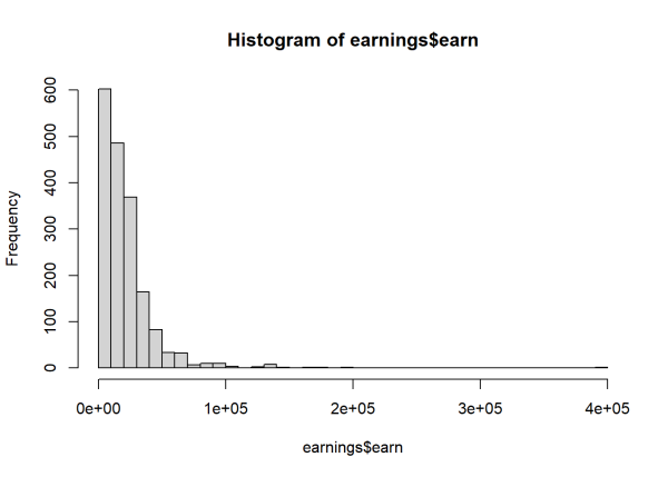
But notice we get an error when we try to model a log-transformed outcome.

m <- lm(log(earn) ~ education + female, data = earnings)

Error in lm.fit(x, y, offset = offset, singular.ok = singular.ok, ...): NA/NaN/Inf in 'y'

This is because we have zeroes in our outcome. Quite a few, in fact.

sum(earnings$earn == 0)

[1] 187

If we want to log-transform the outcome in our model, we either need to drop those rows with 0 earnings, or add a small constant amount to all earnings so we no longer have zeroes.1 We demonstrate the former approach using the subset argument in the lm() function.

m <- lm(log(earn) ~ education + female, data = earnings, subset = earn > 0) summary(m)

Call: lm(formula = log(earn) ~ education + female, data = earnings, subset = earn > 0) Residuals: Min 1Q Median 3Q Max -4.5237 -0.3860 0.1323 0.5148 3.0406 Coefficients: Estimate Std. Error t value Pr(>|t|) (Intercept) 8.504663 0.111317 76.40 <2e-16 *** education 0.112833 0.007949 14.19 <2e-16 *** female -0.487998 0.041493 -11.76 <2e-16 *** --- Signif. codes: 0 '***' 0.001 '**' 0.01 '*' 0.05 '.' 0.1 ' ' 1 Residual standard error: 0.8213 on 1624 degrees of freedom Multiple R-squared: 0.1768, Adjusted R-squared: 0.1758 F-statistic: 174.4 on 2 and 1624 DF, p-value: < 2.2e-16

This works but is not ideal since so many of the zeroes are associated with female subjects.

sum(earnings$earn == 0 & earnings$female == 1)

[1] 172

172 of the 187 zeroes, over 90%, belong to females. That’s a lot of data to drop, especially when we’re investigating the association of sex with earnings.

Now let’s see how we can use a Tweedie model to preserve the zeroes. One way to fit a Tweedie model is using the gam() function from the {mgcv} package. This package is part of the base R installation so you shouldn’t need to install it. The formula syntax is identical to the lm() syntax. The only difference is the family argument where we specify the outcome takes a Tweedie distribution (tw) with a log link. We call the log transformation a “link” because it links us back to the linear model. The linear predictor for a Tweedie model is the exponential function, which works with negative or positive values, including 0. The log function is the inverse of the exponential and therefore “links” the linear model to the response, even if the response is a 0. (If you found this explanation of the log link confusing, you may find this brief article helpful.)

library(mgcv) m2 <- gam(earn ~ education + female, data = earnings, family = tw(link = "log")) summary(m2)

Family: Tweedie(p=1.365) Link function: log Formula: earn ~ education + female Parametric coefficients: Estimate Std. Error t value Pr(>|t|) (Intercept) 8.620280 0.107675 80.06 <2e-16 *** education 0.122682 0.007475 16.41 <2e-16 *** female -0.610894 0.037879 -16.13 <2e-16 *** --- Signif. codes: 0 '***' 0.001 '**' 0.01 '*' 0.05 '.' 0.1 ' ' 1 R-sq.(adj) = 0.194 Deviance explained = 21.1% -REML = 18315 Scale est. = 352.28 n = 1814

Notice the model summary reports using all the data to fit the model (n = 1814). Because we used all the data, the coefficient for female is much bigger. In the linear model where we dropped the zeroes and log-transformed income, the female coefficient is about -0.49. To interpret, we exponentiate and get 0.61. This says among people with the same level of education, earnings for females are about 39% lower than males. (1 - 0.61 = 0.39)

1 - exp(coef(m)["female"])

female 0.3861458

In the Tweedie model, the female coefficient is about -0.61. After exponentiating, this says among people with the same level of education, earnings for females are about 46% lower than males. (1 - 0.54 = 0.46) That’s a notable difference!

1 - exp(coef(m2)["female"])

female 0.4571346

Clearly there is a subjective decision about whether to keep people with 0 earnings in our model. There may be good reasons to drop them. We should also note the R squared in both models is relatively low, which says neither model does a great job of explaining variation in earnings. We would be wise to interpret these coefficients with caution. And of course this data is quite old and we’re only using it for educational purposes. However, at the time of this writing, the gender pay gap in the US is unfortunately very real.

Tweedie model details

Now let’s dig into Tweedie models and learn more about how they work. To begin, they are named after the British statistician, Maurice Tweedie, who first studied the probability distributions that would come to bear his name. The family of Tweedie distributions has variance of the form $\text{var}[Y] = \phi\mu^{p}$. This says the variance is connected to the mean ($\mu$) raised to a power ($p$) and multiplied by a dispersion parameter ($\phi$). Of particular interest are distributions with values of $p$ in the interval (1,2). This produces distributions that can produce zeroes as well as positive, continuous values.

We can use the rtweedie() function from the {tweedie} package to generate random values from a Tweedie distribution. You’ll need to install this package using install.packages("tweedie"). Below we sample 1000 values from a Tweedie distribution with $\mu$ = 2, and variance = $(2.5)2^{1.4}$.

library(tweedie) set.seed(99) y <- rtweedie(n = 1000, phi = 2.5, mu = 2, power = 1.4) summary(y)

Min. 1st Qu. Median Mean 3rd Qu. Max. 0.0000 0.0000 0.9904 2.0395 3.2005 16.4327

Notice this distribution returns positive, continuous values as well as quite a few zeroes. A histogram reveals an excessive amount of zeroes relative to the rest of the data.

hist(y, breaks = 50)

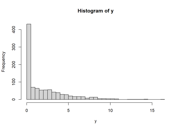
If we pretend this data was given to us and we wanted to model it as a Tweedie distribution, we could fit an intercept-only model using the gam() function as follows:

m0 <- gam(y ~ 1, family = tw(link = "log")) summary(m0)

Family: Tweedie(p=1.389) Link function: log Formula: y ~ 1 Parametric coefficients: Estimate Std. Error t value Pr(>|t|) (Intercept) 0.71268 0.04113 17.33 <2e-16 *** --- Signif. codes: 0 '***' 0.001 '**' 0.01 '*' 0.05 '.' 0.1 ' ' 1 R-sq.(adj) = 0 Deviance explained = 2.23e-12% -REML = 1997 Scale est. = 2.6158 n = 1000

In the summary output we see the power parameter ($p$) is estimated to be 1.389, close to the 1.4 we used to generate the data. The estimated dispersion parameter ($\phi$) labeled “Scale est.”, is 2.6158, not too far off from the true value of 2.5. And the estimated mean is the exponentiated intercept, which is very close to the true value of 2:

exp(coef(m0))

(Intercept) 2.039455

We can visually compare our theoretical and estimated Tweedie distributions using the dtweedie() function (also from the {tweedie} package) along with the curve() function. Notice the close agreement and spike at 0.

curve(dtweedie(x, phi = 2.5, mu = 2, power = 1.4), ylab = "Probability density", from = 0, to = 16, ) curve(dtweedie(x, phi = 2.6158, mu = 2.039455, power = 1.389), add = TRUE, lty = 2) legend("topright", legend = c("Theoretical", "Estimated"), lty = c(1, 2))

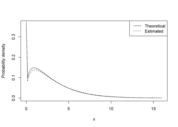
Comparison of theoretical and estimated Tweedie distributions.

Because of their ability to generate excessive zeroes, Tweedie models might be thought of as zero-inflated models for continuous data. Though it’s important to note that, unlike zero-inflated models for count data, Tweedie models do not allow you to separately model the zero-generating process.

When values of $p$ range from 1 to 2, the Tweedie distribution is actually a compound Poisson-Gamma distribution (Faraway 2016). To be precise, observations are generated by summing draws from a gamma distribution, but the number of gamma observations to sum is itself a draw from a Poisson distribution. Recall that the Poisson distribution is specified by its mean ($\lambda$) and that the gamma distribution is specified by its shape ($\alpha$) and scale ($\sigma$) parameters. When specified in terms of $p$, $\phi$, and $\mu$, it turns out the Poisson mean is given by

\[ \lambda = \mu^{2 - p}/((2-p)\phi) \tag{1} \]

Likewise, the gamma shape and scale parameters are given by

\[ \alpha = (2-p)/(p-1) \tag{2} \]

\[ \sigma = \phi(p-1)\mu^{p-1} \tag{3} \]

Using R we can easily generate this process. Below we sample 1 value from a Tweedie distribution with $\mu$ = 2, and variance = $(2.5)2^{1.4}$ (i.e., $\phi$ = 2.5 and $p$ = 1.4).

set.seed(321) # make result replicable p <- 1.4 phi <- 2.5 mu <- 2 # how many gamma draws? N <- rpois(n = 1, lambda = mu^(2 - p)/(phi * (2 - p))) N

[1] 3

# sample N gamma draws X <- rgamma(n = N, shape = (2 - p)/(p - 1), scale = phi*(p - 1)*mu^(p - 1)) X

[1] 4.116106 0.593558 1.166353

# sum the N gamma draws Y <- sum(X) Y

[1] 5.876017

This particular draw sampled a 5.876017. But notice that the draw from the Poisson distribution could produce a 0, which would mean 0 draws from a Gamma distribution, and thus a final value of 0. Hence why the Tweedie distribution can be useful for modeling continuous responses that can sometimes be 0.

We can use the replicate() function and implement our own version of the rtweedie() function we used above to sample 1000 values.

samp <- replicate(n = 1e4, expr = { N <- rpois(n = 1, lambda = mu^(2 - p)/(phi * (2 - p))) X <- rgamma(n = N, shape = (2 - p)/(p - 1), scale = phi*(p - 1)*mu^(p - 1)) Y <- sum(X) Y }) summary(samp)

Min. 1st Qu. Median Mean 3rd Qu. Max. 0.000 0.000 1.080 1.997 3.136 26.560

The rtweedie() function from the {tweedie} package is more efficient than our implementation, but digging into this process allows us to see that the probability of getting a zero can be estimated using the Poisson distribution.

The probability of drawing a certain count, $k$, from a Poisson distribution with mean $\lambda$ is

\[ P(X = k) = \frac{\lambda^ke^{-\lambda}}{k!} \tag{4} \]

The probability of drawing a 0 simplifies this expression to

\[ P(X = 0) = e^{-\lambda} \tag{5} \]

Let’s use this expression to estimate the probability of drawing a zero from the Tweedie distribution we sampled above.

The mean of the Poisson of the process is $\mu^{2 - p}/((2-p)\phi)$. When we plug in our parameters of $\mu = 2$, $p = 1.4$, and $\phi = 2.5$, this is $2^{2 - 1.4}/((2-1.4)2.5) = 1.010478$. Therefore the probability of drawing a zero count is

\[P(X = 0) = e^{-1.010478} \approx 0.36\]

This can be calculated using the dpois() function:

dpois(x = 0, lambda = 1.010478)

[1] 0.3640449

We can also estimate the probability of drawing a 0 by simply taking the proportion of zeroes in our sample. This is in close agreement to the theoretical probability.

mean(y == 0)

[1] 0.381

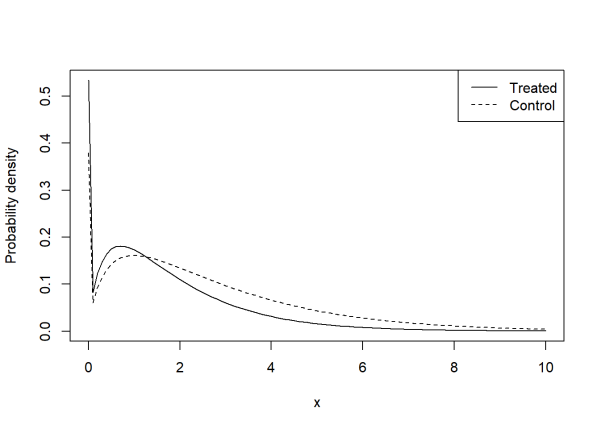
What if we make the mean of our Tweedie distribution conditional on other variables? Perhaps there is one distribution for a treated group and another for a control group. We can simulate this scenario by creating a variable consisting of zeroes and ones, where 0 is control and 1 is treated, and modifying the mean based on that variable. Below we use the expression 0.5 + -0.6*trt to set a mean of 0.5 for the control group and a mean of -0.1 for the treated group. This a linear model with an intercept of 0.5 and a slope coefficient of -0.6. Notice we wrap the expression in the exp() function. This exponentiates the result and ensures it is positive. So the means are actually exp(0.5) = 1.649 and exp(-0.1) = 0.904. This is why we need the log link for the Tweedie distribution. The log “undoes” the exponentiation and is thus our “link” to the original linear model. When finished, we place the simulated data in a data frame and use {ggplot2} to create histograms of the outcomes for each group. We can see the treated group has many more zeroes.

n <- 1000 set.seed(11) trt <- sample(0:1, size = n, replace = TRUE) y2 <- rtweedie(n = 1000, phi = 2.5, mu = exp(0.5 + -0.6*trt), power = 1.4) d <- data.frame(y2, trt = factor(trt, labels = c("control", "treated"))) library(ggplot2) ggplot(d) + aes(x = y2) + geom_histogram(bins = 30) + facet_wrap(~trt)

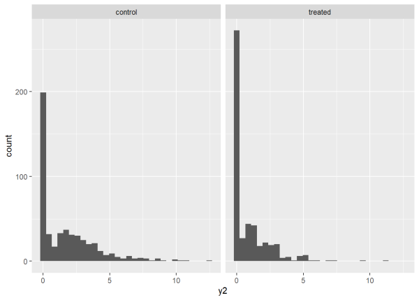
Comparison of control and treated outcome histograms

As before, we can fit a Tweedie model to this data and see how well it estimates the true linear model values of 0.5 and -0.6. In the syntax below we are fitting the exact model we used to simulate the data.

m01 <- gam(y2 ~ trt, family = tw(link = "log")) summary(m01)

Family: Tweedie(p=1.363) Link function: log Formula: y2 ~ trt Parametric coefficients: Estimate Std. Error t value Pr(>|t|) (Intercept) 0.56506 0.05657 9.990 < 2e-16 *** trt -0.68055 0.09096 -7.482 1.61e-13 *** --- Signif. codes: 0 '***' 0.001 '**' 0.01 '*' 0.05 '.' 0.1 ' ' 1 R-sq.(adj) = 0.0518 Deviance explained = 5.05% -REML = 1668.5 Scale est. = 2.3244 n = 1000

Both estimated coefficients are close to the true values and easily within two standard errors. The estimated mean for the control group is the exponentiated intercept. The estimated mean for the treated group is the exponentiated sum of the coefficients.

# control and treated means means <- c(exp(coef(m01)[1]), "trt" = exp(sum(coef(m01)))) means

(Intercept) trt 1.7595543 0.8909302

To estimate the probability of getting a zero in each group, we can use the estimated means as well as the estimated $p$ and $\phi$ values to estimate the means of the Poisson process for each group. We can then use dpois() to estimate the probability of getting a zero for each group. We calculate lambda using Eq. 1 from above.

lambda <- means^(2 - 1.363)/((2 - 1.363) * 2.3244) dpois(x = 0, lambda = lambda)

(Intercept) trt 0.3798455 0.5339354

The estimated probabilities are extremely close to the observed proportions of zeroes in each group.

tapply(y2, trt, function(x)mean(x == 0))

0 1 0.3786982 0.5334686

Finally we can visually compare the estimated Tweedie distributions for each group. Notice the bigger spike at 0 for the treated group.

curve(dtweedie(x, phi = 2.3244, mu = means[2], power = 1.363), ylab = "Probability density", from = 0, to = 10) curve(dtweedie(x, phi = 2.3244, mu = means[1], power = 1.363), add = TRUE, lty = 2) legend("topright", legend = c("Treated", "Control"), lty = c(1, 2))

Comparison of treated and control Tweedie distributions

Returning to the earnings example

Let’s look again at our Tweedie model for the earnings data:

summary(m2)

Setting aside the low R squared, this is telling us the estimated Tweedie distribution of earnings depends on level of education and sex of the subject. The estimated values of $p$ and $\phi$ are 1.365 and 352.28, respectively. The estimated value of $\mu$ depends on level of education and sex. For example, the estimated earnings for a female and male with education level 12 is estimated as follows:

# set type = "response" to get estimate on original scale pred <- predict(m2, newdata = data.frame(education = 12, female = c(1, 0)), type = "response") pred

1 2 13115.69 24160.11

We can use these values and the estimated $p$ and $\phi$ values to estimate the mean of the Poisson process for this Tweedie distribution (Eq. 1):

lambda <- pred^(2 - 1.365)/((2 - 1.365) * 352.28) lambda

1 2 1.841347 2.713976

And now we can estimate the probability of zero earnings for a female and male with education level 12, which turns out to be about 0.16 and 0.06, respectively.

dpois(x = 0, lambda = lambda)

1 2 0.15860368 0.06627275

We can also compare these distributions using the dtweedie() function. However the spike at 0 is so big relative to the rest of the distribution that it only makes sense to compare the curves for the positive values. To make this plot, we generate the probability densities for females and males using the dtweedie() function on the range of \$1 to \$100,000. We then put the values into a data frame and label each group of values as “female” and “male”. Finally we create the plot using the {ggplot2} package.

x <- 1:1e5 y <- c(dtweedie(x, phi = 352.28, mu = pred[1], power = 1.365), dtweedie(x, phi = 352.28, mu = pred[2], power = 1.365)) d <- data.frame(x, y, sex = rep(c("Female", "Male"), each = 1e5)) ggplot(d) + aes(x, y, linetype = sex) + geom_line() + scale_x_continuous(labels = scales::dollar, breaks = seq(0,100000,by =20000)) + labs(x = "Annual earnings", y = "Probability density") + theme_minimal()

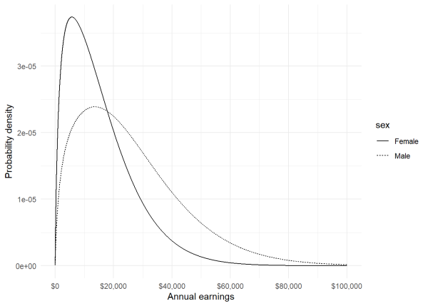
Estimated probability distributions of earnings for males and females with 12 years of education

We see a higher probability for more females to earn less than \$20,000, but higher probability for males to earn more than \$20,000.

As always, before we become too invested in these estimates, we should check some model diagnostics. Since this is technically a GAM model, we need to use the gam.check() function from the {mgcv} package.

par(mfrow = c(2,2)) gam.check(m2)

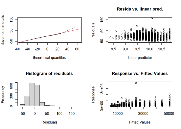
The top right plot shows a great deal of variability in the residuals versus fitted values. This implies model-predicted earnings are very uncertain. The bottom right plot shows predicted values versus observed values. A good fitting model should show a high positive linear relationship, which we do not see here. In fact, if we calculate the correlation of this plot and square the result, we essentially calculate the R squared value. We previously saw this was quite low. All things considered, we probably need more that just education and sex to explain the variability in earnings. Nevertheless, the Tweedie model allowed us to incorporate the zero values of earnings even as we log-transformed it, and allowed us to gain some insight into those subjects with 0 earnings.

Fitting a Tweedie model using glm()

It is possible to use the base R glm() function to fit Tweedie models. This may be desirable if you prefer to work in the GLM framework. One approach is to use the tweedie() function from the {statmod} package. Notice we have to provide a value for $p$. Below we use the value estimated by the gam() function above. Setting link.power = 0 says we want to use a “log” link. Notice the coefficients are very similar to those estimated using the GAM approach, though the estimate for $\phi$ is a good deal higher at 463.8472.

# install.packages("statmod") library(statmod) # for tweedie() m3 <- glm(earn ~ education + female, data = earnings, family = tweedie(var.power = 1.365, link.power = 0)) summary(m3)

Call: glm(formula = earn ~ education + female, family = tweedie(var.power = 1.365, link.power = 0), data = earnings) Coefficients: Estimate Std. Error t value Pr(>|t|) (Intercept) 8.620282 0.123582 69.75 <2e-16 *** education 0.122681 0.008579 14.30 <2e-16 *** female -0.610895 0.043475 -14.05 <2e-16 *** --- Signif. codes: 0 '***' 0.001 '**' 0.01 '*' 0.05 '.' 0.1 ' ' 1 (Dispersion parameter for Tweedie family taken to be 463.8472) Null deviance: 945927 on 1813 degrees of freedom Residual deviance: 746276 on 1811 degrees of freedom AIC: NA Number of Fisher Scoring iterations: 5

We could also estimate $p$ separately using the tweedie.profile() function from the {tweedie} package. Be warned this function can be pretty slow. See its help page for tips on speeding up the estimation. The estimated value for $p$ will be in the “xi.max” element. (In the literature, the Greek letter “xi”, $\xi$, is often used in place of $p$.)

p_est <- tweedie.profile(earn ~ education + female, data = earnings) p_est$xi.max

[1] 1.359184

And then we can use this estimate directly in the tweedie() function.

m3 <- glm(earn ~ education + female, data = earnings, family = tweedie(var.power = p_est$xi.max, link.power = 0)) summary(m3)

Call: glm(formula = earn ~ education + female, family = tweedie(var.power = p_est$xi.max, link.power = 0), data = earnings) Coefficients: Estimate Std. Error t value Pr(>|t|) (Intercept) 8.620074 0.123598 69.74 <2e-16 *** education 0.122693 0.008578 14.30 <2e-16 *** female -0.610807 0.043461 -14.05 <2e-16 *** --- Signif. codes: 0 '***' 0.001 '**' 0.01 '*' 0.05 '.' 0.1 ' ' 1 (Dispersion parameter for Tweedie family taken to be 491.3603) Null deviance: 999486 on 1813 degrees of freedom Residual deviance: 787901 on 1811 degrees of freedom AIC: NA Number of Fisher Scoring iterations: 5

You may have noticed the AIC is missing in the model summary output. That’s because Tweedie models require special handling to compute the AIC. Fortunately, the {tweedie} package provides the AICtweedie() helper function to calculate this.

AICtweedie(m3)

[1] 36655.17

It’s worth noting you can also use the {glmmTMB} package to fit Tweedie models. Here’s how to fit our model using the glmmTMB() function. The model summary automatically includes an AIC value as well as other fit statistics.

# install.packages("glmmTMB") library(glmmTMB) m4 <- glmmTMB(earn ~ education + female, data = earnings, family = tweedie(link = 'log')) summary(m4)

Family: tweedie ( log ) Formula: earn ~ education + female Data: earnings AIC BIC logLik deviance df.resid 36621.3 36648.8 -18305.7 36611.3 1809 Dispersion parameter for tweedie family (): 353 Conditional model: Estimate Std. Error z value Pr(>|z|) (Intercept) 8.620277 0.106694 80.79 <2e-16 *** education 0.122682 0.007414 16.55 <2e-16 *** female -0.610891 0.037833 -16.15 <2e-16 *** --- Signif. codes: 0 '***' 0.001 '**' 0.01 '*' 0.05 '.' 0.1 ' ' 1

To see the estimated value of the power parameter, you need to use the family_params() function on the fitted model object.

family_params(m4)

Tweedie power 1.364596

Hopefully this article has helped you get started with Tweedie models. We recommend you explore the references below to learn more, in particular chapter 9 of Faraway (2016) and chapter 3 of Wood (2017).

References

Mollie E. Brooks, Kasper Kristensen, Koen J. van Benthem, Arni Magnusson, Casper W. Berg, Anders Nielsen, Hans J. Skaug, Martin Maechler and Benjamin M. Bolker (2017). glmmTMB Balances Speed and Flexibility Among Packages for Zero-inflated Generalized Linear Mixed Modeling. The R Journal, 9(2), 378-400. doi: 10.32614/RJ-2017-066. glmmTMB R package version 1.1.10.
Dunn, P. K. (2022). Tweedie: Evaluation of Tweedie exponential family models. R package version 2.3.
Gelman A, Hill J, and Vehtari A. (2020). Regression and Other Stories. Cambridge University Press.
Faraway, J. (2016). Extending the Linear Model with R (2nd edition). CRC Press. (Chapter 9)
R Core Team (2024). R: A Language and Environment for Statistical Computing. R Foundation for Statistical Computing, Vienna, Austria. https://www.R-project.org/. Version 4.4.3.
Ross, C. E. (1996) WORK, FAMILY, AND WELL-BEING IN THE UNITED STATES, 1990 Computer file. Champaign, IL: University of Illinois, Survey Research Laboratory producer, 1995. Ann Arbor, MI: Inter-university Consortium for Political and Social Research distributor.
Smyth, G, et al. (2022). Statistical Modeling. R package version 1.5.0.
Wickham, H. (2016) ggplot2: Elegant Graphics for Data Analysis. Springer-Verlag New York. ggplot2 R package version 3.5.1.
Wikipedia contributors, “Tweedie distribution,” Wikipedia, The Free Encyclopedia, https://en.wikipedia.org/w/index.php?title=Tweedie_distribution&oldid=1278490429 (accessed March 14, 2025).
Wood, S.N. (2017) Generalized Additive Models: An Introduction with R (2nd edition). Chapman and Hall/CRC. (Chapter 3) mgcv R package version 1.9-1.

Clay Ford
Statistical Research Consultant
University of Virginia Library
March 26, 2025

Adding a small constant, c, to a variable so it can be log transformed can be difficult to justify, though it seems to be a common procedure. The amount you add can have a lot of influence on the transformed values, so it needs to be chosen with care. For example, adding c = 1 to a 0 results in a log transformation of 0. Adding c = 0.0001 to a 0 results in a log transformation of about -9.2. In some cases performing a log(x + c) transformation results in a strange bimodal distribution with a spike at the transformed zeroes. We encourage the interested reader to experiment with hist(log(earnings$earn + c)) with various values of c to see an example.??

For questions or clarifications regarding this article, contact statlab@virginia.edu.

View the entire collection of UVA Library StatLab articles, or learn how to cite.