One of the basic assumptions of linear modeling is constant, or homogeneous, variance. What does that mean exactly? Let’s simulate some data that satisfies this condition to illustrate the concept.
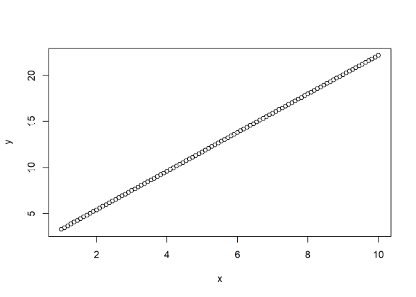
Below we create a sorted vector of numbers ranging from 1 to 10 called x, and then create a vector of numbers called y that is a function of x. When we plot x vs y, we get a straight line with an intercept of 1.2 and a slope of 2.1.
x <- seq(1,10, length.out = 100)
y <- 1.2 + 2.1 * x
plot(x, y)
Now let’s add some “noise” to our data so that y is not completely determined by x. We can do that by randomly drawing values from a theoretical normal distribution with mean 0 and some set variance, and then adding them to the formula that generates y. The rnorm() function in R allows us to easily do this. Below we draw 100 random values from a normal distribution with mean 0 and standard deviation 2 and save as a vector called noise. (Recall that standard deviation is simply the square root of variance.) Then we generate y with the noise added. The function set.seed(222) allows you to get the same “random” data in case you want to follow along. Finally we re-plot the data.
set.seed(222)
noise <- rnorm(n = 100, mean = 0, sd = 2)
y <- 1.2 + 2.1 * x + noise
plot(x, y)
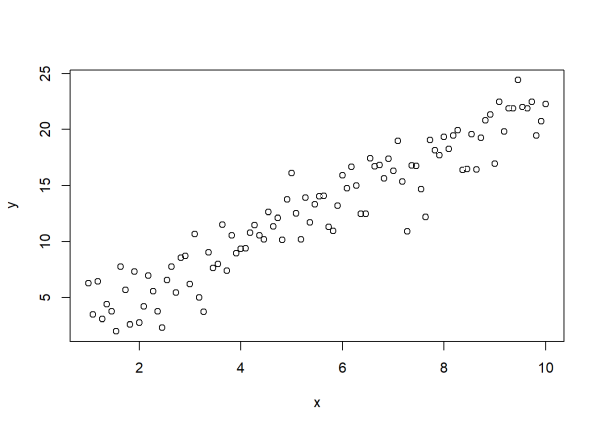
Now we have data that are a combination of a linear, deterministic component (\(y = 1.2 + 2.1x\)) and random noise drawn from a \(N(0, 2)\) distribution. These are the basic assumptions we make about our data when we fit a traditional linear model. Below we use the lm() function to “recover” the “true” values we used to generate the data, of which there are three:
- The intercept: 1.2
- The slope: 2.1
- The standard deviation: 2
m <- lm(y ~ x)
summary(m)
  Call:
  lm(formula = y ~ x)

  Residuals:
      Min      1Q  Median      3Q     Max
  -5.5831 -1.2165  0.3288  1.3022  4.3714

  Coefficients:
              Estimate Std. Error t value Pr(>|t|)
  (Intercept)  1.27426    0.44720   2.849  0.00534 **
  x            2.09449    0.07338  28.541  < 2e-16 ***
  ---
  Signif. codes:  0 '***' 0.001 '**' 0.01 '*' 0.05 '.' 0.1 ' ' 1

  Residual standard error: 1.926 on 98 degrees of freedom
  Multiple R-squared:  0.8926, Adjusted R-squared:  0.8915
  F-statistic: 814.6 on 1 and 98 DF,  p-value: < 2.2e-16
The intercept and slope estimates in the "Coefficients" section, 1.27 and 2.09, are quite close to 1.2 and 2.1, respectively. The residual standard error of 1.926 is also quite close to the constant value of 2. We produced a “good” model because we knew how y was generated and gave the lm() function the “correct” model to fit. While we can’t do this in real life, it’s a useful exercise to help us understand the assumptions of linear modeling.
Now what if the variance was not constant? What if we multiplied the standard deviation of 2 by the square root of x? As we see in the plot below, the vertical scatter of the points increases as x increases.
set.seed(222)
noise <- rnorm(n = 100, mean = 0, sd = 2 * sqrt(x))
y <- 1.2 + 2.1 * x + noise
plot(x, y)
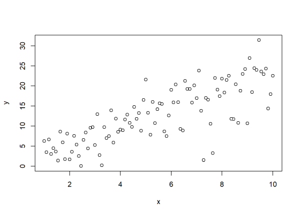
We multiplied 2 by sqrt(x) because we’re specifying standard deviation. If we could specify variance, we would have multiplied 4 by just x.
If we fit the same model using lm(), we get a residual standard error of 4.488.
m2 <- lm(y ~ x)
summary(m2)
  Call:
  lm(formula = y ~ x)

  Residuals:
       Min       1Q   Median       3Q      Max
  -15.0460  -2.4013   0.5638   2.8734  10.2996

  Coefficients:
              Estimate Std. Error t value Pr(>|t|)
  (Intercept)    1.313      1.042    1.26    0.211
  x              2.096      0.171   12.26   <2e-16 ***
  ---
  Signif. codes:  0 '***' 0.001 '**' 0.01 '*' 0.05 '.' 0.1 ' ' 1

  Residual standard error: 4.488 on 98 degrees of freedom
  Multiple R-squared:  0.6051, Adjusted R-squared:  0.6011
  F-statistic: 150.2 on 1 and 98 DF,  p-value: < 2.2e-16
We know that isn’t right, because we simulated the data. There was no constant standard deviation when we created the “noise.” Each random value was drawn from a different normal distribution, each with mean 0 but a standard deviation that varied according to x. This means our assumption of constant variance is violated. How would we detect this in real life?
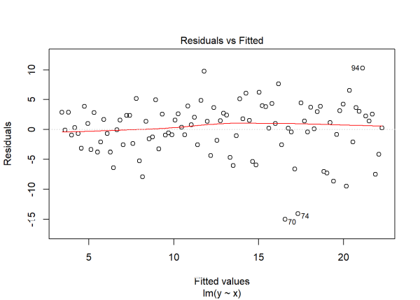
The most common way is plotting residuals versus fitted values. This is easy to do in R. Just call plot() on the model object. This generates four different plots to assess the traditional modeling assumptions. See this blog post for more information. The plots we’re interested in are the 1st and 3rd plots, which we can specify with the which argument.
plot(m2, which = 1)
plot(m2, which = 3)
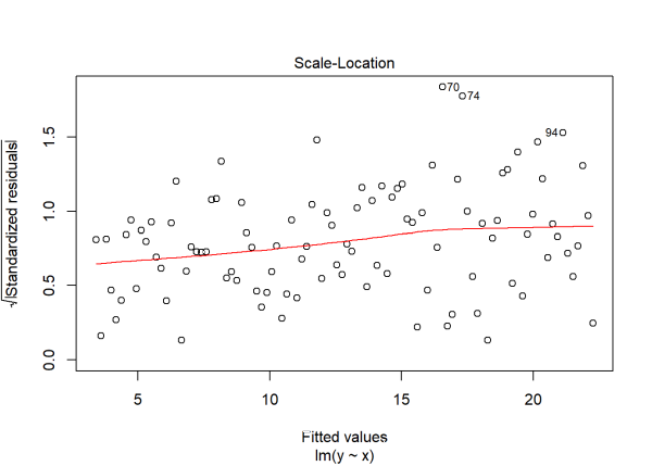
In the first plot we see the variability around 0 increase as we move further to the right with bigger fitted values. In the third plot we also see increasing variability as we move to the right, though this time the residuals have been standardized and transformed to the square root scale. The positive trajectory of the smooth red line indicates an increase in variance.
So now that we’ve confirmed that our assumption of non-constant variance is invalid, what can we do? One approach is to log transform the data. This sometimes works if your response variable is positive and highly skewed. But that’s not really the case here. y is only slightly skewed. (Call hist() on y to verify.) Plus, we know our data are not on a log scale.
Another approach is to model the non-constant variance. That’s the topic of this blog post.
To do this, we will use functions from the nlme package that is included with the base installation of R. The workhorse function is gls(), which stands for “generalized least squares.” We use it just as we would the lm() function, except we also use the weights argument along with a handful of variance functions. Let’s demonstrate with an example.
Below we fit the “correct” model to our data that exhibited non-constant variance. We load the nlme package so we can use the gls() function.1 We specify the model syntax as before, y ~ x. Then we use the weights argument to specify the variance function, in this case varFixed(), also part of the nlme package. This says our variance function has no parameters and a single covariate, x, which is precisely how we generated the data. The syntax, ~x, is a one-sided formula that can be read as “model variance as a function of x.”
library(nlme)
vm1 <- gls(y ~ x, weights = varFixed(~x))
summary(vm1)
  Generalized least squares fit by REML
    Model: y ~ x
    Data: NULL
         AIC      BIC    logLik
    576.2928 584.0477 -285.1464

  Variance function:
   Structure: fixed weights
   Formula: ~x

  Coefficients:
                 Value Std.Error   t-value p-value
  (Intercept) 1.369583 0.6936599  1.974431  0.0511
  x           2.085425 0.1504863 13.857900  0.0000

   Correlation:
    (Intr)
  x -0.838

  Standardized residuals:
         Min         Q1        Med         Q3        Max
  -2.8942967 -0.6293867  0.1551594  0.6758773  2.2722755

  Residual standard error: 1.925342
  Degrees of freedom: 100 total; 98 residual
The result produces a residual standard error of 1.925 that is very close to 2, the “true” value we used to generate the data. The intercept and slope values, 1.37 and 2.09, are also very close to 1.2 and 2.1.
Once again we can call plot() on the model object. In this case only one plot is generated: standardized residuals versus fitted values:
plot(vm1)
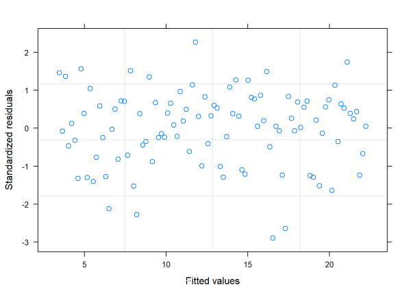
This plot looks good. As long as we model our variance as a function of x, the fitted model neither overfits nor underfits in any systematic sort of way (unlike when we used lm() to fit the model and assumed constant variance.)
The varFixed() function creates weights for each observation, symbolized as \(w_i\). The idea is that the higher the weight a given observation has, the smaller the variance of the normal distribution from which its noise component was drawn. In our example, as x increases the variance increases. Therefore higher weights should be associated with smaller x values. This can be accomplished by taking the reciprocal of x, that is \(w_i = 1/x\). So when \(x = 2\), \(w = 1/2\). When \(x = 10\), \(w = 1/10\). Larger x get smaller weights.
Finally, to ensure larger weights are associated with smaller variances, we divide the constant variance by the weight. Stated mathematically,
\[\epsilon_i \sim N(0, \sigma^2/w_i)\]
Or taking the square root to express standard deviation,
\[\epsilon_i \sim N(0, \sigma/ \sqrt{w_i})\]
So the larger the denominator (i.e., the larger the weight and, hence, the smaller the x), the smaller the variance and more precise the observed y.
Incidentally, we can use lm() to weight observations as well. It too has a weights argument like the gls() function. The only difference is we have to be more explicit about how we express the weights. In this case, we have to specify the reciprocal of x. Notice the result is almost identical to what we get using gls() and varFixed().
m3 <- lm(y ~ x, weights = 1/x)
summary(m3)
  Call:
  lm(formula = y ~ x, weights = 1/x)

  Weighted Residuals:
      Min      1Q  Median      3Q     Max
  -5.5725 -1.2118  0.2987  1.3013  4.3749

  Coefficients:
              Estimate Std. Error t value Pr(>|t|)
  (Intercept)   1.3696     0.6937   1.974   0.0511 .
  x             2.0854     0.1505  13.858   <2e-16 ***
  ---
  Signif. codes:  0 '***' 0.001 '**' 0.01 '*' 0.05 '.' 0.1 ' ' 1

  Residual standard error: 1.925 on 98 degrees of freedom
  Multiple R-squared:  0.6621, Adjusted R-squared:  0.6587
  F-statistic:   192 on 1 and 98 DF,  p-value: < 2.2e-16
The power of the nlme package is that it allows a variety of variance functions. The varFixed() function we just illustrated is the simplest and something that can be done with lm(). The other variance functions include:
varIdent()varPower()varExp()varConstPower()varComb()
Let’s explore each of these using simulated data.
varIdent()
The varIdent() function allows us to model different variances per stratum. To see how it works, we’ll first simulate data with this property. Below we use set.seed(11) in case someone wants to simulate the same random data. Then we set n equal to 400, the number of observations we will simulate. x is generated the same as before. In this example, we include an additional predictor called g which can be thought of as gender. We randomly sample 400 values of “m” and “f”. Next we simulate a vector of two standard deviations and save it as msd. If g == "m", then the standard deviation is \(2 \times 2.5\). Otherwise it’s \(2\) for g == "f". We use this vector in the next line to generate y. Notice where msd is plugged into the rnorm function. Also notice how we generate y. We include an interaction between x and y. When g == "f", the intercept and slope is 1.2 and 2.1. When g == "m", the intercept and slope are (1.2 + 2.8) and (2.1 + 2.8), respectively. Finally we place our simulated data into a data frame and plot with ggplot2.
set.seed(11)
n <- 400
x <- seq(1,10, length.out = n)
g <- sample(c("m","f"), size = n, replace = TRUE)
msd <- ifelse(g=="m", 2*2.5, 2)
y <- 1.2 + 2.1*x - 1.5*(g == "m") + 2.8*x*(g == "m") + rnorm(n, sd = msd)
d <- data.frame(y, x, g)

library(ggplot2)
ggplot(d, aes(x, y, color = g)) +
  geom_point()
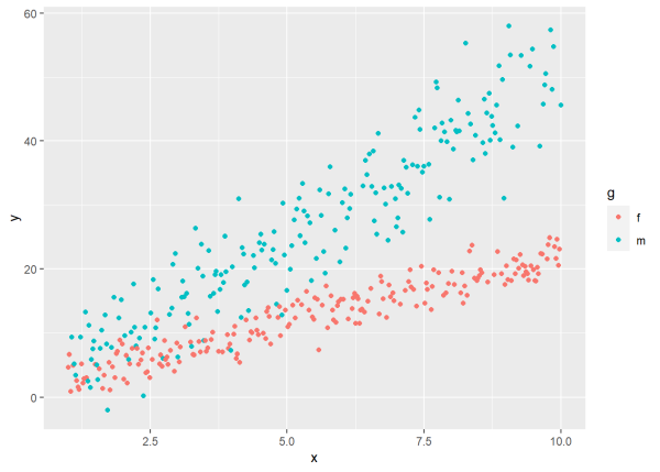
Notice the different variances for each level of g. The variance for “m” is much greater than the variance for “f”. It has a lot more scatter than “f”. We simulated the data that way. We set the variance for “m” to be 2.5 times that of “f”.
Now let’s use the gls() function with varIdent() in attempt to recover these true values. We follow the same approach as before, defining our variance function in the weights argument. Below we specify in the form argument that the formula for modeling variance is conditional on g. The expression ~ 1|g is a one-sided formula that says the variance differs between the levels of g. The 1 just means we have no additional covariates in our model for variance. It is possible to include a formula such as ~ x|g, but that would be incorrect in this case since we did not use x in generating the variance. Looking at the plot also shows that while the variability in y is different between the groups, the variability does not increase as x increases.
vm2 <- gls(y ~ x*g, data = d, weights = varIdent(form = ~ 1|g))
summary(vm2)
  Generalized least squares fit by REML
    Model: y ~ x * g
    Data: d
         AIC     BIC    logLik
    2081.752 2105.64 -1034.876

  Variance function:
   Structure: Different standard deviations per stratum
   Formula: ~1 | g
   Parameter estimates:
        f       m
  1.00000 2.58127

  Coefficients:
                   Value Std.Error  t-value p-value
  (Intercept)  0.9686349 0.3237724  2.99172  0.0029
  x            2.1222707 0.0525024 40.42239  0.0000
  gm          -1.9765090 0.9352152 -2.11343  0.0352
  x:gm         2.9957974 0.1553551 19.28355  0.0000

   Correlation:
       (Intr) x      gm
  x    -0.901
  gm   -0.346  0.312
  x:gm  0.304 -0.338 -0.907

  Standardized residuals:
          Min          Q1         Med          Q3         Max
  -2.74115039 -0.67013954  0.01619031  0.69793776  2.72985748

  Residual standard error: 2.005397
  Degrees of freedom: 400 total; 396 residual
First, notice at the bottom of the output that the estimated residual standard error is 2.005397, very close to the “true” value of 2. Also notice in the “Variance function” section we get an estimated value of 2.58127 for group “m”, which is very close to the “true” value of 2.5 we used to generate the different variance for group “m”. In general, when you use the varIdent() function to estimate different variances between levels of strata, one of the levels will be set to baseline, and the others will be estimated as multiples of the residual standard error. In this case since “f” comes before “m” alphabetically, “f” was set to baseline, or 1. The estimated residual standard error for group “f” is \(2.005397 \times 1\). The estimated residual standard error for group “m” is \(2.005397 \times 2.58127\).
It’s important to note these are just estimates. To get a feel for the uncertainty of these estimates, we can use the intervals() function from the nlme package to get 95% confidence intervals. To reduce the output, we save the result and view selected elements of the object.
int <- intervals(vm2)
The varStruct element contains the 95% confidence interval for the parameter estimated in the variance function. The parameter in this case is the residual standard error multiplier for the male group.
int$varStruct
       lower    est.    upper
  m 2.245615 2.58127 2.967095
  attr(,"label")
  [1] "Variance function:"
The sigma element contains the 95% confidence interval for the residual standard error.
int$sigma
     lower     est.    upper
  1.818639 2.005397 2.211335
  attr(,"label")
  [1] "Residual standard error:"
Both intervals are quite small and contain the “true” value we used to generate the data.
varPower()
The varPower() function allows us to model variance as a power of the absolute value of a covariate. Once again, to help explain this we will simulate data with this property. Below, the main thing to notice is the sd argument of the rnorm() function. That’s where we take the standard deviation of 2 and then multiply it by the absolute value of x raised to the power of 1.5. This is similar to how we simulated data to demonstrate the varFixed() function above. In that case we simply assumed the exponent was 0.5. (Recall taking the square root of a number is equivalent to raising it to the power of 0.5.) Here we arbitrarily picked a power of 1.5. When we use gls() with varPower() we will attempt to recover the “true” value of 1.5 in addition to 2.
set.seed(4)
n <- 1000
x <- seq(1,10,length.out = n)
y <- 1.2 + 2.1*x + rnorm(n, sd = 2*abs(x)^1.5)
d <- data.frame(y, x)
ggplot(d, aes(x, y)) + geom_point()

We see the data exhibiting the classic form of variance increasing as the predictor increases. To correctly model this data using gls(), we supply it with the formula y ~ x and use the weights argument with varPower(). Notice we specify the one-sided formula just as we did with the varFixed() function. In this model, however, we’ll get an estimate for the power.
vm3 <- gls(y ~ x, data = d, weights = varPower(form = ~x))
summary(vm3)
  Generalized least squares fit by REML
    Model: y ~ x
    Data: d
         AIC      BIC    logLik
    8840.188 8859.811 -4416.094

  Variance function:
   Structure: Power of variance covariate
   Formula: ~x
   Parameter estimates:
     power
  1.520915

  Coefficients:
                 Value Std.Error  t-value p-value
  (Intercept) 2.321502 0.4750149 4.887218       0
  x           1.582272 0.2241367 7.059404       0

   Correlation:
    (Intr)
  x -0.845

  Standardized residuals:
           Min           Q1          Med           Q3          Max
  -2.892319514 -0.655237190  0.001653178  0.691241690  3.346273816

  Residual standard error: 1.872944
  Degrees of freedom: 1000 total; 998 residual
int <- intervals(vm3)
int$varStruct
           lower     est.    upper
  power 1.445064 1.520915 1.596765
  attr(,"label")
  [1] "Variance function:"
int$sigma
     lower     est.    upper
  1.650987 1.872944 2.124740
  attr(,"label")
  [1] "Residual standard error:"
The power is estimated to be 1.52 which is very close to the “true” value of 1.5. The estimated residual standard error of 1.872944 is also quite close to 2. Both intervals capture the values we used to simulate the data. The coefficients in the model, on the other hand, are somewhat poorly estimated. This is not surprising given how much variability is in y, especially for \(x > 2\).
varExp()
The varExp() function allows us to model variance as an exponential function of a covariate. Yet again we’ll explain this variance function using simulated data. The only change is in the sd argument of the rnorm() function. We have a fixed value of 2 that we multiply by x which is itself multiplied by 0.5 and exponentiated. Notice how rapidly the variance increases as we increase x. This is due to the exponential growth of the variance.
set.seed(55)
n <- 400
x <- seq(1, 10, length.out = n)
y <- 1.2 + 2.1*x + rnorm(n, sd = 2*exp(0.5*x))
d <- data.frame(y, x)
ggplot(d, aes(x, y)) + geom_point()
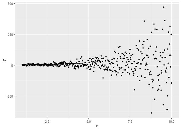
To work backwards and recover these values, we use the varExp() function in the weights argument of gls(). The one-sided formula does not change in this case. It says model the variance as a function of x. The varExp() function says that x has been multiplied by some value and exponentiated, so gls() will try to estimate that value.
vm4 <- gls(y ~ x, data = d, weights = varExp(form = ~x))
summary(vm4)
  Generalized least squares fit by REML
    Model: y ~ x
    Data: d
         AIC      BIC    logLik
    3873.153 3889.098 -1932.576

  Variance function:
   Structure: Exponential of variance covariate
   Formula: ~x
   Parameter estimates:
      expon
  0.4845623

  Coefficients:
                 Value Std.Error  t-value p-value
  (Intercept) 1.198525 1.1172841 1.072713   0.284
  x           2.073297 0.4933502 4.202486   0.000

   Correlation:
    (Intr)
  x -0.892

  Standardized residuals:
          Min          Q1         Med          Q3         Max
  -3.16976627 -0.69525696  0.00614222  0.63718022  2.90423217

  Residual standard error: 2.119192
  Degrees of freedom: 400 total; 398 residual
int <- intervals(vm4)
int$varStruct
            lower      est.     upper
  expon 0.4562871 0.4845623 0.5128374
  attr(,"label")
  [1] "Variance function:"
int$sigma
     lower     est.    upper
  1.786737 2.119192 2.513505
  attr(,"label")
  [1] "Residual standard error:"
The “expon” estimate of 0.4845623 in the “Variance function” section is very close to our specified value of 0.5. Likewise, the estimated residual standard error of 2.119192 is close to the “true” value of 2. The model coefficient estimates are also close to the values we used to generate the data, but notice the uncertainty in the intercept. The hypothesis test in the summary can’t rule out a negative intercept. This again is not surprising since y has so much non-constant variance and since we have no observations of x equal to 0. Since the intercept is the value y takes when x equals 0, our estimated intercept is an extrapolation to an event we did not observe.
varConstPower()
The varConstPower() function allows us to model variance as a positive constant plus a power of the absolute value of a covariate. That’s a mouthful, but this is basically the same as the varPower() function except now we add a positive constant to it. The following code simulates data for which the varConstPower() function would be suitable to use. Notice it is identical to the code we used to simulate data for the varPower() section, except we add 0.7 to abs(x)^1.5. Why 0.7? No special reason. It’s just a positive constant we picked.
set.seed(4)
n <- 1000
x <- seq(1,10,length.out = n)
y <- 1.2 + 2.1*x + rnorm(n, sd = 2*(0.7 + abs(x)^1.5))
d <- data.frame(y, x)
ggplot(d, aes(x, y)) + geom_point()
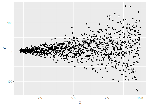
The correct way to model this data is to use gls() with the varConstPower() function. The one-sided formula is the same as before. The summary returns three estimates for the variance model: the constant, the power and the residual standard error. Recall the “true” values are 0.7, 1.5 and 2, respectively.
vm5 <- gls(y ~ x, data = d, weights = varConstPower(form = ~x))
summary(vm5)
Generalized least squares fit by REML
  Model: y ~ x
  Data: d
       AIC      BIC    logLik
  9033.253 9057.782 -4511.627

Variance function:
 Structure: Constant plus power of variance covariate
 Formula: ~x
 Parameter estimates:
    const     power
0.3388157 1.4463162

Coefficients:
               Value Std.Error  t-value p-value
(Intercept) 2.550278 0.6140015 4.153538       0
x           1.527665 0.2517976 6.067037       0

 Correlation:
  (Intr)
x -0.831

Standardized residuals:
         Min           Q1          Med           Q3          Max
-2.843996437 -0.660034231  0.000752882  0.681577120  3.299594323

Residual standard error: 2.199816
Degrees of freedom: 1000 total; 998 residual
int <- intervals(vm5)
int$varStruct
           lower      est.   upper
const 0.03191368 0.3388157 3.59708
power 1.25559225 1.4463162 1.63704
attr(,"label")
[1] "Variance function:"
int$sigma
   lower     est.    upper
1.476361 2.199816 3.277783
attr(,"label")
[1] "Residual standard error:"
The intervals are fairly tight and contain the “true” values we used to generate the data.
varComb()
Finally, the varComb() function allows us to model combinations of two or more variance models by multiplying together the corresponding variance functions. Obviously this can accommodate some very complex variance models. We’ll simulate some basic data that would be appropriate to use with the varComb() function.
What we do below is combine two different variance processes:
- One that allows standard deviation to differ between gender (
“f”= \(2\),“m”= \(2 \times 2.5\)) - One that allows standard deviation to increase as
xincreases, wherexis multiplied by 1.5 and exponentiated
To help with visualizing the data we have limited x to range from 1 to 3.
set.seed(77)
n <- 400
x <- seq(1, 3, length.out = n)
g <- sample(c("m","f"), size = n, replace = TRUE)
msd <- ifelse(g=="m", 2*2.5, 2) * exp(1.5*x)
y <- 1.2 + 2.1*x - 1.5*(g == "m") + 2.8*x*(g == "m") + rnorm(n, sd = msd)
d <- data.frame(y, x, g)
ggplot(d, aes(x, y, color = g)) +
  geom_point()
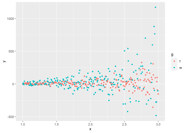
The plot shows increasing variance as x increases, but also differences in variance between genders. The variance of y for group “m” is much greater than the variance of y in group “f”, especially when x is greater than 1.5.
To correctly model the data generating process we specified above and attempt to recover the true values, we use the varComb() function as a wrapper around two more variance functions: varIdent() and varExp(). Why these two? Because we have different variances between genders, and we have variance increasing exponentially as a function of x.
vm6 <- gls(y ~ x*g, data = d,
           weights = varComb(varIdent(form = ~ 1|g),
                             varExp(form = ~x)))
summary(vm6)
  Generalized least squares fit by REML
    Model: y ~ x * g
    Data: d
        AIC     BIC    logLik
    4431.45 4459.32 -2208.725

  Combination of variance functions:
   Structure: Different standard deviations per stratum
   Formula: ~1 | g
   Parameter estimates:
         f        m
  1.000000 2.437046
   Structure: Exponential of variance covariate
   Formula: ~x
   Parameter estimates:
     expon
  1.540608

  Coefficients:
                   Value Std.Error    t-value p-value
  (Intercept)  -5.996337  6.539552 -0.9169339  0.3597
  x             8.829971  4.849272  1.8208860  0.0694
  gm          -17.572238 16.548540 -1.0618603  0.2889
  x:gm         16.932938 12.192793  1.3887661  0.1657

   Correlation:
       (Intr) x      gm
  x    -0.972
  gm   -0.395  0.384
  x:gm  0.387 -0.398 -0.974

  Standardized residuals:
          Min          Q1         Med          Q3         Max
  -2.74441479 -0.67478610 -0.00262221  0.66079254  3.14975288

  Residual standard error: 1.794185
  Degrees of freedom: 400 total; 396 residual
The summary section contains two sections for modeling variance. The first estimates the multiplier for the “m” group to be 2.437, which is very close to the true value of 2.5. The exponential parameter is estimated to be 1.54, extremely close to the true value of 1.5 we used when generating the data. Finally the residual standard error is estimated to be about 1.79, close to the true value of 2. Calling intervals(vm6) shows very tight confidence intervals. The A and B prefixes in the varStruct element are just labels for the two different variance models.
int <- intervals(vm6)
int$varStruct
             lower     est.    upper
  A.m     2.119874 2.437046 2.801673
  B.expon 1.419366 1.540608 1.661850
  attr(,"label")
  [1] "Variance function:"
int$sigma
     lower     est.    upper
  1.380008 1.794185 2.332669
  attr(,"label")
  [1] "Residual standard error:"
Unfortunately, due to the large exponential variability, the estimates of the model coefficients are woefully bad.
What’s the point?
So why did we simulate all this fake data and then attempt to recover “true” values? What good is that? Fair questions. The answer is it helps us understand what assumptions we’re making when we specify and fit a model. When we specify and fit the following model…
m <- lm(y ~ x1 + x2)
…we’re saying we think y is approximately equal to a weighted sum of x1 and x2 (plus an intercept), with errors being random draws from a normal distribution with mean of 0 and some fixed standard deviation. Likewise, if we specify and fit the following model…
m <- gls(y ~ x1 + x2, data = d, weights = varPower(form = ~x1))
…we’re saying we think y is approximately equal to a weighted sum of x1 and x2 (plus an intercept), with errors being random draws from a normal distribution with mean of 0 and a standard deviation that grows as a multiple of x1 raised by some power.
If we can simulate data suitable for those models, then we have a better understanding of the assumptions we’re making when we use those models. Hopefully you now have a better understanding of what you can do to model variance using the nlme package.
R session details
The analysis was done using the R Statistical language (v4.5.1; R Core Team, 2025) on Windows 11 x64, using the packages nlme (v3.1.168) and ggplot2 (v4.0.0).
References
- Pinheiro, J., & Bates, D. (2000). Mixed-effects models in S and S-PLUS. Springer. https://doi.org/10.1007/b98882
- Pinheiro, J., Bates, D., & R Core Team. (2020). nlme: Linear and nonlinear mixed effects models (Version 3.1-162). https://cran.r-project.org/package=nlme
- R Core Team. (2020). R: A language and environment for statistical computing. R Foundation for Statistical Computing. https://www.r-project.org/
- Wickham, H. (2016). ggplot2: Elegant graphics for data analysis. Springer-Verlag.
Clay Ford
Statistical Research Consultant
University of Virginia Library
April 7, 2020
- The nlme package is perhaps better known for its
lme()function, which is used to fit mixed-effect models (i.e., models with both fixed and random effects). This blog post demonstrates variance functions usinggls(), which does not fit random effects. However, everything we present in this blog post can be used withlme(). ↩
For questions or clarifications regarding this article, contact statlab@virginia.edu.
View the entire collection of UVA Library StatLab articles, or learn how to cite.
